Lecture 7: Recommender Systems Part I

UBC Master of Data Science program, 2024-25

People who agreed in the past are likely to agree again in future.
– The Master Algorithm

Imports and LOs

Imports

import os
import random
import sys
import time

import numpy as np
import pandas as pd

import matplotlib.pyplot as plt
from sklearn.decomposition import PCA
from sklearn.model_selection import cross_validate, train_test_split

plt.rcParams["font.size"] = 12

%matplotlib inline
pd.set_option("display.max_colwidth", 0)

DATA_DIR = os.path.join(os.path.abspath(".."), "data/")
sys.path.append(os.path.join(os.path.abspath(".."), "code"))

---------------------------------------------------------------------------
ImportError                               Traceback (most recent call last)
Cell In[1], line 10
      7 import pandas as pd
      9 import matplotlib.pyplot as plt
---> 10 from sklearn.decomposition import PCA
     11 from sklearn.model_selection import cross_validate, train_test_split
     13 plt.rcParams["font.size"] = 12

File ~/miniforge3/envs/jbook/lib/python3.12/site-packages/sklearn/__init__.py:73
     62 # `_distributor_init` allows distributors to run custom init code.
     63 # For instance, for the Windows wheel, this is used to pre-load the
     64 # vcomp shared library runtime for OpenMP embedded in the sklearn/.libs
   (...)
     67 # later is linked to the OpenMP runtime to make it possible to introspect
     68 # it and importing it first would fail if the OpenMP dll cannot be found.
     69 from . import (  # noqa: F401 E402
     70     __check_build,
     71     _distributor_init,
     72 )
---> 73 from .base import clone  # noqa: E402
     74 from .utils._show_versions import show_versions  # noqa: E402
     76 _submodules = [
     77     "calibration",
     78     "cluster",
   (...)
    114     "compose",
    115 ]

File ~/miniforge3/envs/jbook/lib/python3.12/site-packages/sklearn/base.py:19
     17 from ._config import config_context, get_config
     18 from .exceptions import InconsistentVersionWarning
---> 19 from .utils._estimator_html_repr import _HTMLDocumentationLinkMixin, estimator_html_repr
     20 from .utils._metadata_requests import _MetadataRequester, _routing_enabled
     21 from .utils._param_validation import validate_parameter_constraints

File ~/miniforge3/envs/jbook/lib/python3.12/site-packages/sklearn/utils/__init__.py:15
     13 from . import _joblib, metadata_routing
     14 from ._bunch import Bunch
---> 15 from ._chunking import gen_batches, gen_even_slices
     16 from ._estimator_html_repr import estimator_html_repr
     18 # Make _safe_indexing importable from here for backward compat as this particular
     19 # helper is considered semi-private and typically very useful for third-party
     20 # libraries that want to comply with scikit-learn's estimator API. In particular,
     21 # _safe_indexing was included in our public API documentation despite the leading
     22 # `_` in its name.

File ~/miniforge3/envs/jbook/lib/python3.12/site-packages/sklearn/utils/_chunking.py:11
      8 import numpy as np
     10 from .._config import get_config
---> 11 from ._param_validation import Interval, validate_params
     14 def chunk_generator(gen, chunksize):
     15     """Chunk generator, ``gen`` into lists of length ``chunksize``. The last
     16     chunk may have a length less than ``chunksize``."""

File ~/miniforge3/envs/jbook/lib/python3.12/site-packages/sklearn/utils/_param_validation.py:14
     11 from numbers import Integral, Real
     13 import numpy as np
---> 14 from scipy.sparse import csr_matrix, issparse
     16 from .._config import config_context, get_config
     17 from .validation import _is_arraylike_not_scalar

File ~/miniforge3/envs/jbook/lib/python3.12/site-packages/scipy/sparse/__init__.py:315
    312 from ._sputils import get_index_dtype, safely_cast_index_arrays
    314 # For backward compatibility with v0.19.
--> 315 from . import csgraph
    317 # Deprecated namespaces, to be removed in v2.0.0
    318 from . import (
    319     base, bsr, compressed, construct, coo, csc, csr, data, dia, dok, extract,
    320     lil, sparsetools, sputils
    321 )

File ~/miniforge3/envs/jbook/lib/python3.12/site-packages/scipy/sparse/csgraph/__init__.py:187
    158 __docformat__ = "restructuredtext en"
    160 __all__ = ['connected_components',
    161            'laplacian',
    162            'shortest_path',
   (...)
    184            'csgraph_to_masked',
    185            'NegativeCycleError']
--> 187 from ._laplacian import laplacian
    188 from ._shortest_path import (
    189     shortest_path, floyd_warshall, dijkstra, bellman_ford, johnson, yen,
    190     NegativeCycleError
    191 )
    192 from ._traversal import (
    193     breadth_first_order, depth_first_order, breadth_first_tree,
    194     depth_first_tree, connected_components
    195 )

File ~/miniforge3/envs/jbook/lib/python3.12/site-packages/scipy/sparse/csgraph/_laplacian.py:7
      5 import numpy as np
      6 from scipy.sparse import issparse
----> 7 from scipy.sparse.linalg import LinearOperator
      8 from scipy.sparse._sputils import convert_pydata_sparse_to_scipy, is_pydata_spmatrix
     11 ###############################################################################
     12 # Graph laplacian

File ~/miniforge3/envs/jbook/lib/python3.12/site-packages/scipy/sparse/linalg/__init__.py:129
      1 """
      2 Sparse linear algebra (:mod:`scipy.sparse.linalg`)
      3 ==================================================
   (...)
    126 
    127 """
--> 129 from ._isolve import *
    130 from ._dsolve import *
    131 from ._interface import *

File ~/miniforge3/envs/jbook/lib/python3.12/site-packages/scipy/sparse/linalg/_isolve/__init__.py:4
      1 "Iterative Solvers for Sparse Linear Systems"
      3 #from info import __doc__
----> 4 from .iterative import *
      5 from .minres import minres
      6 from .lgmres import lgmres

File ~/miniforge3/envs/jbook/lib/python3.12/site-packages/scipy/sparse/linalg/_isolve/iterative.py:5
      3 from scipy.sparse.linalg._interface import LinearOperator
      4 from .utils import make_system
----> 5 from scipy.linalg import get_lapack_funcs
      7 __all__ = ['bicg', 'bicgstab', 'cg', 'cgs', 'gmres', 'qmr']
     10 def _get_atol_rtol(name, b_norm, atol=0., rtol=1e-5):

File ~/miniforge3/envs/jbook/lib/python3.12/site-packages/scipy/linalg/__init__.py:203
      1 """
      2 ====================================
      3 Linear algebra (:mod:`scipy.linalg`)
   (...)
    200 
    201 """  # noqa: E501
--> 203 from ._misc import *
    204 from ._cythonized_array_utils import *
    205 from ._basic import *

File ~/miniforge3/envs/jbook/lib/python3.12/site-packages/scipy/linalg/_misc.py:3
      1 import numpy as np
      2 from numpy.linalg import LinAlgError
----> 3 from .blas import get_blas_funcs
      4 from .lapack import get_lapack_funcs
      6 __all__ = ['LinAlgError', 'LinAlgWarning', 'norm']

File ~/miniforge3/envs/jbook/lib/python3.12/site-packages/scipy/linalg/blas.py:213
    210 import numpy as np
    211 import functools
--> 213 from scipy.linalg import _fblas
    214 try:
    215     from scipy.linalg import _cblas

ImportError: dlopen(/Users/kvarada/miniforge3/envs/jbook/lib/python3.12/site-packages/scipy/linalg/_fblas.cpython-312-darwin.so, 0x0002): Library not loaded: @rpath/libgfortran.5.dylib
  Referenced from: <0B9C315B-A1DD-3527-88DB-4B90531D343F> /Users/kvarada/miniforge3/envs/jbook/lib/libopenblas.0.dylib
  Reason: tried: '/Users/kvarada/miniforge3/envs/jbook/lib/libgfortran.5.dylib' (duplicate LC_RPATH '@loader_path'), '/Users/kvarada/miniforge3/envs/jbook/lib/libgfortran.5.dylib' (duplicate LC_RPATH '@loader_path'), '/Users/kvarada/miniforge3/envs/jbook/lib/python3.12/site-packages/scipy/linalg/../../../../libgfortran.5.dylib' (duplicate LC_RPATH '@loader_path'), '/Users/kvarada/miniforge3/envs/jbook/lib/python3.12/site-packages/scipy/linalg/../../../../libgfortran.5.dylib' (duplicate LC_RPATH '@loader_path'), '/Users/kvarada/miniforge3/envs/jbook/bin/../lib/libgfortran.5.dylib' (duplicate LC_RPATH '@loader_path'), '/Users/kvarada/miniforge3/envs/jbook/bin/../lib/libgfortran.5.dylib' (duplicate LC_RPATH '@loader_path'), '/usr/local/lib/libgfortran.5.dylib' (no such file), '/usr/lib/libgfortran.5.dylib' (no such file, not in dyld cache)

Lecture plan

• Motivation (~10 mins)

• Formulating the recommendation problem (~10 mins)

• Evaluation and baseline approaches (~10 mins)

• Questions for class discussion (~5 mins)

• Break (~5 mins)

• Collaborative filtering (~20 mins)

• Class demo (~10 mins)

• Questions for class discussion (~5 mins)

• Summary and conclusion (~5 mins)

Learning outcomes

From this lecture, students are expected to be able to:

• State the problem of recommender systems.

• Describe components of a utility matrix.

• Create a utility matrix given ratings data.

• Describe a common approach to evaluate recommender systems.

• Implement some baseline approaches to complete the utility matrix.

• Explain the idea of collaborative filtering.

• Describe how you can use a PCA-like model to fill in the utility matrix.

• Explain how to interpret \(Z\) and \(W\) in the context of recommendation systems.

• Explain how the loss function of collaborative filtering differs from the loss function of regular PCA.

• Learn to be mindful of some serious consequences of recommendation systems.

❓❓ Questions for you

What percentage of watch time on YouTube do you think comes from recommendations?

• (A) 50%

• (B) 60%

• (C) 20%

• (D) 90%

This question is based on this source. The statistics might have changed now.

1. Recommender systems intro and motivation

1.1 What is a recommender system?

• A recommender or a recommendation system recommends a particular product or service to users they are likely to consume.

Example: Recommender Systems

• A user goes to Amazon to buy products.

• Amazon has some information about the user. They also have information about other users buying similar products.

• What should they recommend to the user, so that they buy more products?

• There’s no “right” answer (no label).

• The whole idea is to understand user behavior in order to recommend them products they are likely to consume.

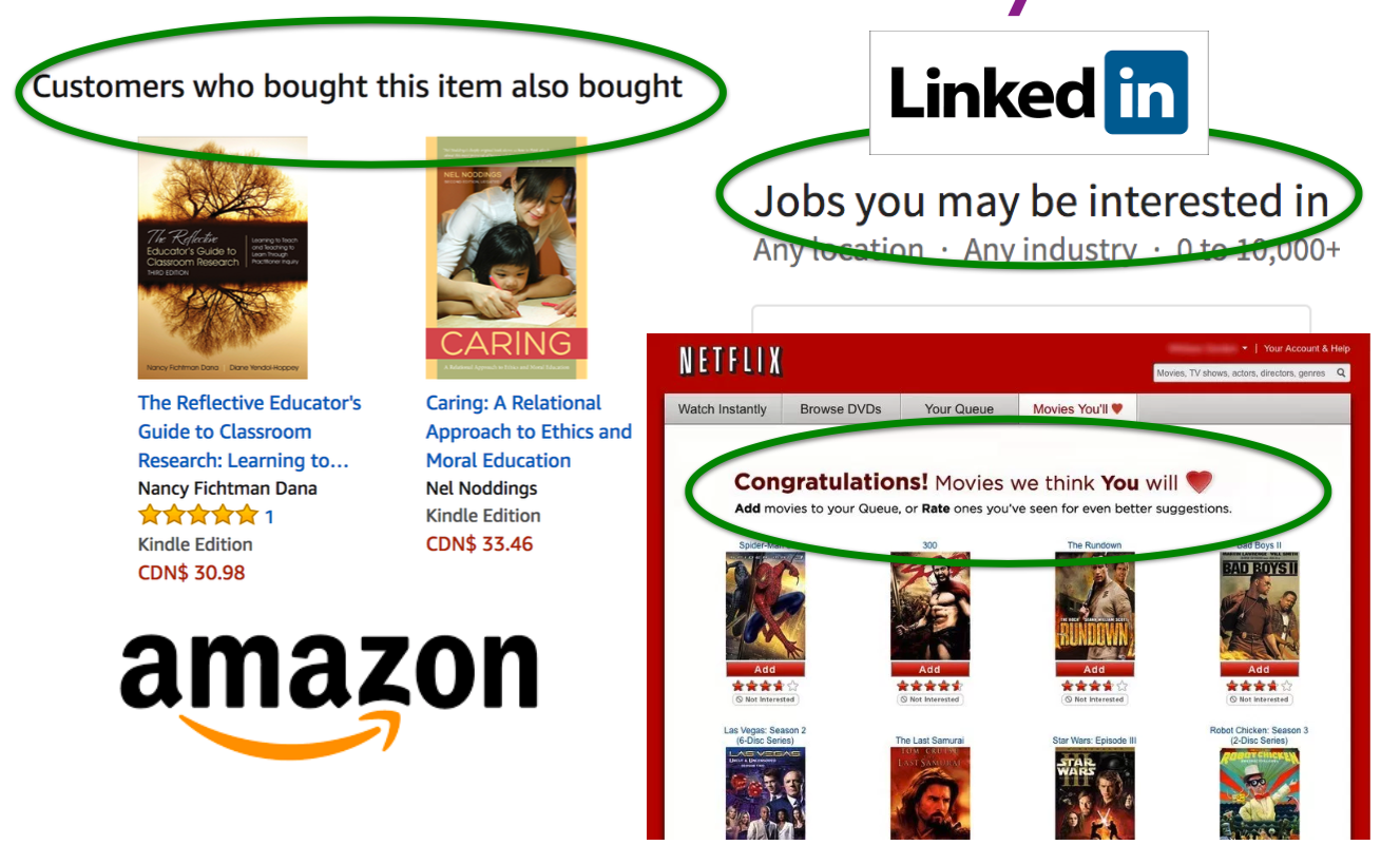
1.2 Why should we care about recommendation systems?

• Almost everything we buy or consume today is in some way or the other influenced by recommendation systems.

  • Music (Spotify), videos (YouTube), news, books and products (Amazon), movies (Netflix), jokes, restaurants, dating , friends (Facebook), professional connections (LinkedIn)

• Recommendation systems are at the core of the success of many companies such as Amazon and Netflix.

• As a result, we receive Capstone projects focused on developing recommender systems.

  • A Past MDS Capstone: Present personalized journal article recommendations to health care professionals.

• Recommendation systems are often presented as powerful tools that significantly reduce the effort users need to put in finding items, effectively mitigating the problem of information overload.

• This is more or less true in many contexts. Consider, for instance, the experience of shopping an umbrella on Amazon without the help of recommendations or any specific ranking of products.

• In the absence of a recommendation system, users would be faced with the daunting task of sifting through thousands of available products to find the one that best suits their needs.

• That said, we should always be mindful of the drawbacks of relying heavily on recommender systems.

• For example, these systems tend to recommend articles and products that are similar to those a user has previously interacted with or those their friends like.

• While this can improve user experience by presenting more of what the system predicts the user will like, it can also lead to a phenomenon known as “filter bubbles”.

• This effect narrows a user’s exposure to diverse viewpoints and information. Such a narrowing of perspective can be detrimental, particularly in the context of scientific research or political discourse, where exposure to a wide range of perspectives is crucial.

1.3 Data and main approaches

What kind of data we need to build recommendation systems?

• User-item interactions (e.g., ratings or clicks) (most common)

• Features related to items or users

• Customer purchase history data

Main approaches

• Collaborative filtering (today’s focus)

  • “Unsupervised” learning

  • We only have labels \(y_{ij}\) (rating of user \(i\) for item \(j\)).

  • We learn latent features.

• Content-based recommenders

  • Supervised learning

  • Extract features \(x_i\) of users and/or items building a model to predict rating \(y_i\) given \(x_i\).

  • Apply model to predict for new users/items.

• Hybrid

  • Combining collaborative filtering with content-based filtering

2. Recommender systems problem

2.1 Problem formulation

• Most often the data for recommender systems come in as interactions between a set of items and a set of users.

• We have two entities: \(N\) users and \(M\) items.

• Users are consumers.

• Items are the products or services offered.

  • E.g., movies (Netflix), books (Amazon), songs (spotify), people (tinder)

• A utility matrix is the matrix that captures interactions between \(N\) users and \(M\) items.

• The interaction may come in different forms:

  • ratings, clicks, purchases

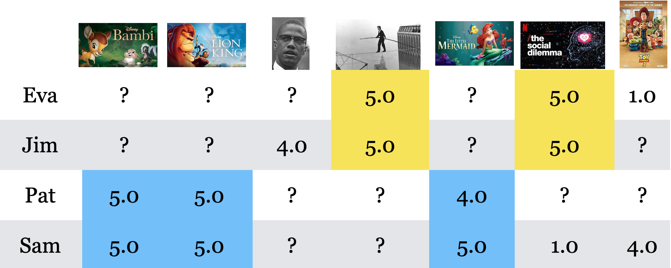
• Below is a toy utility matrix. Here \(N\) = 6 and \(M\) = 5.

• Each entry \(y_{ij}\) (\(i^{th}\) row and \(j^{th}\) column) denotes the rating given by the user \(i\) to item \(j\).

• We represent users in terms of items and items in terms of users.

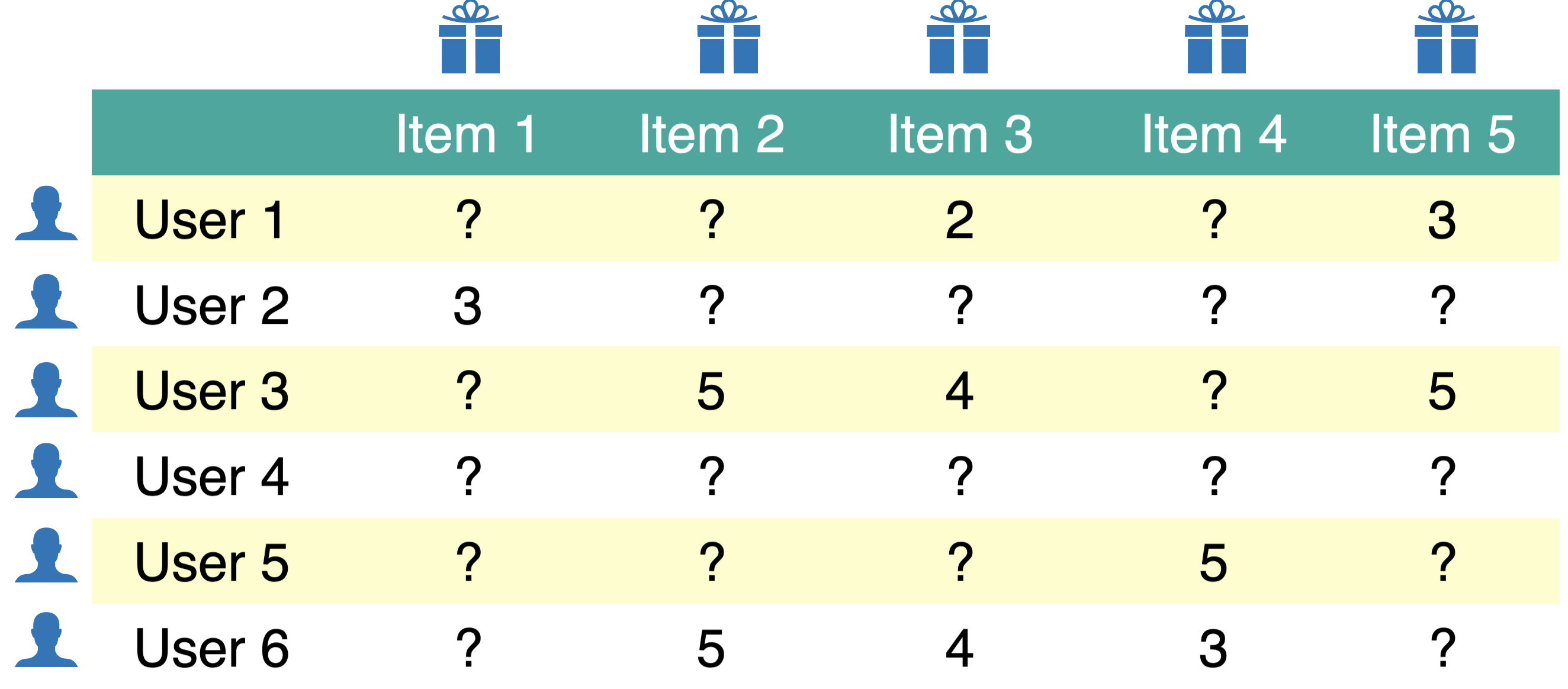
• The utility matrix is very sparse because usually users only interact with a few items.

• For example:

  • all Netflix users will have rated only a small percentage of content available on Netflix

  • all amazon clients will have rated only a small fraction of items among all items available on Amazon

What do we predict?

Given a utility matrix of \(N\) users and \(M\) items, complete the utility matrix. In other words, predict missing values in the matrix.

• Once we have predicted ratings, we can recommend items to users they are likely to rate higher.

• Note: rating prediction \(\neq\) Classification or regression

In classification or regression:

• We have \(X\) and targets for some rows in \(X\).

• We want to predict the last column (target column).

\[\begin{split} \begin{bmatrix} \checkmark & \checkmark & \checkmark & \checkmark & \checkmark\\ \checkmark & \checkmark & \checkmark & \checkmark & \checkmark\\ \checkmark & \checkmark & \checkmark & \checkmark & \checkmark\\ \checkmark & \checkmark & \checkmark & \checkmark & ?\\ \checkmark & \checkmark & \checkmark & \checkmark & ?\\ \checkmark & \checkmark & \checkmark & \checkmark & ?\\ \end{bmatrix} \end{split}\]

In rating prediction

• Ratings data has many missing values in the utility matrix. There is no special target column. We want to predict the missing entries in the matrix.

• Since our goal is to predict ratings, usually the utility matrix is referred to as \(Y\) matrix.

\[\begin{split} \begin{bmatrix} ? & ? & \checkmark & ? & \checkmark\\ \checkmark & ? & ? & ? & ?\\ ? & \checkmark & \checkmark & ? & \checkmark\\ ? & ? & ? & ? & ?\\ ? & ? & ? & \checkmark & ?\\ ? & \checkmark & \checkmark & ? & \checkmark \end{bmatrix} \end{split}\]

2.2 Creating utility matrix

Let’s work with the following toy example.

toy_ratings = pd.read_csv(DATA_DIR + "toy-movie-ratings.csv")
toy_ratings

	user_id	movie_id	rating
0	Sam	Lion King	5
1	Sam	Toy Story	4
2	Sam	The Little Mermaid	5
3	Sam	Bambi	5
4	Sam	The Social Dilemma	1
5	Eva	Toy Story	1
6	Eva	The Social Dilemma	5
7	Eva	Man on Wire	5
8	Pat	The Little Mermaid	4
9	Pat	Lion King	5
10	Pat	Bambi	5
11	Jim	The Social Dilemma	5
12	Jim	Malcolm x	4
13	Jim	Man on Wire	5

Here is the utility matrix.

Let’s try to build it using Python.

user_key = "user_id"
item_key = "movie_id"

def get_stats(ratings, item_key="movie_id", user_key="user_id"):
    print("Number of ratings:", len(ratings))
    print("Average rating:  %0.3f" % (np.mean(ratings["rating"])))
    N = len(np.unique(ratings[user_key]))
    M = len(np.unique(ratings[item_key]))
    print("Number of users (N): %d" % N)
    print("Number of items (M): %d" % M)
    print("Fraction non-nan ratings: %0.3f" % (len(ratings) / (N * M)))
    return N, M


N, M = get_stats(toy_ratings)

Number of ratings: 14
Average rating:  4.214
Number of users (N): 4
Number of items (M): 7
Fraction non-nan ratings: 0.500

• Let’s construct utility matrix with number of users rows and number of items columns from the ratings data.

Note we are constructing a non-sparse matrix for demonstration purpose here. In real life it’s recommended that you work with sparse matrices.

user_mapper = dict(zip(np.unique(toy_ratings[user_key]), list(range(N))))
item_mapper = dict(zip(np.unique(toy_ratings[item_key]), list(range(M))))
user_inverse_mapper = dict(zip(list(range(N)), np.unique(toy_ratings[user_key])))
item_inverse_mapper = dict(zip(list(range(M)), np.unique(toy_ratings[item_key])))

• Why do we need all these mappers?

  • We want to store the rating for user \(i\) and item \(j\) at \(Y[i,j]\) location in the utility matrix.

  • So we define user_mapper and item_mapper which map user and item ids to indices.

  • Once we have predicted ratings for users and items, we want to be able to map it to the original user and item ids so that we recommend the right product to the right user.

  • So we have user_inverse_mapper and item_inverse_mapper which map indices to original user and item ids.

def create_Y_from_ratings(
    data, N, M, user_mapper, item_mapper, user_key="user_id", item_key="movie_id"
):  # Function to create a dense utility matrix
    Y = np.zeros((N, M))
    Y.fill(np.nan)
    for index, val in data.iterrows():
        n = user_mapper[val[user_key]]
        m = item_mapper[val[item_key]]
        Y[n, m] = val["rating"]

    return Y

Y_mat = create_Y_from_ratings(toy_ratings, N, M, user_mapper, item_mapper)
Y_mat.shape

(4, 7)

pd.DataFrame(Y_mat)

	0	1	2	3	4	5	6
0	NaN	NaN	NaN	5.0	NaN	5.0	1.0
1	NaN	NaN	4.0	5.0	NaN	5.0	NaN
2	5.0	5.0	NaN	NaN	4.0	NaN	NaN
3	5.0	5.0	NaN	NaN	5.0	1.0	4.0

• Rows represent users.

• Columns represent items (movies in our case).

• Each cell gives the rating given by the user to the corresponding movie.

• Users are features for movies and movies are features for users.

• Our goal is to predict missing entries in the utility matrix.

2.3 Evaluation

• We’ll try a number of methods to fill in the missing entries in the utility matrix.

• Although there is no notion of “accurate” recommendations, we need a way to evaluate our predictions so that we’ll be able to compare different methods.

• Although we are doing unsupervised learning, we’ll split the data and evaluate our predictions as follows.

Data splitting

• We split the ratings into train and validation sets.

• It’s easier to split the ratings data instead of splitting the utility matrix.

• Don’t worry about y; we’re not really going to use it.

X = toy_ratings.copy()
y = toy_ratings[user_key]
X_train, X_valid, y_train, y_valid = train_test_split(
    X, y, test_size=0.2, random_state=42
)

X_train.shape, X_valid.shape

((11, 3), (3, 3))

Now we will create utility matrices for train and validation splits.

train_mat = create_Y_from_ratings(X_train, N, M, user_mapper, item_mapper)
valid_mat = create_Y_from_ratings(X_valid, N, M, user_mapper, item_mapper)

train_mat.shape, valid_mat.shape

((4, 7), (4, 7))

(len(X_train) / (N * M)) # Fraction of non-nan entries in the train set

0.39285714285714285

(len(X_valid) / (N * M)) # Fraction of non-nan entries in the valid set

0.10714285714285714

pd.DataFrame(train_mat)

	0	1	2	3	4	5	6
0	NaN	NaN	NaN	5.0	NaN	5.0	1.0
1	NaN	NaN	4.0	5.0	NaN	NaN	NaN
2	5.0	NaN	NaN	NaN	4.0	NaN	NaN
3	5.0	NaN	NaN	NaN	5.0	1.0	4.0

pd.DataFrame(valid_mat)

	0	1	2	3	4	5	6
0	NaN	NaN	NaN	NaN	NaN	NaN	NaN
1	NaN	NaN	NaN	NaN	NaN	5.0	NaN
2	NaN	5.0	NaN	NaN	NaN	NaN	NaN
3	NaN	5.0	NaN	NaN	NaN	NaN	NaN

• train_mat has only ratings from the train set and valid_mat has only ratings from the valid set.

• During training we assume that we do not have access to some of the available ratings. We predict these ratings and evaluate them against ratings in the validation set.

❓❓ Questions for you

• Why are utility matrices for train and validation sets are of the same shape?

• Now that we have train and validation sets, how do we evaluate our predictions?

• You can calculate the error between actual ratings and predicted ratings with metrics of your choice.

  • Most common ones are MSE or RMSE.

• The error function below calculates RMSE and evaluate function prints train and validation RMSE.

• Lower RMSE \(\rightarrow\) predicted ratings are closer to the actual ratings

def error(X1, X2):
    """
    Returns the root mean squared error.
    """
    return np.sqrt(np.nanmean((X1 - X2) ** 2))


def evaluate(pred_X, train_X, valid_X, model_name="Global average"):
    print("%s train RMSE: %0.2f" % (model_name, error(pred_X, train_X)))
    print("%s valid RMSE: %0.2f" % (model_name, error(pred_X, valid_X)))

❓❓ Questions for you

• Can we use this method to evaluate predicted ratings that are not available to us?

3. Baseline Approaches

Let’s first try some simple approaches to predict missing entries.

1. Global average baseline

2. Per-user average baseline

3. Per-item average baseline

4. Average of 2 and 3

   • Take an average of per-user and per-item averages.

5. \(k\)-Nearest Neighbours imputation

I’ll show you 1. and 5. You’ll explore 2., 3., and 4. in the lab.

3.1 Global average baseline

• Let’s examine RMSE of the global average baseline.

• In this baseline we predict everything as the global average rating.

avg = np.nanmean(train_mat)
pred_g = np.zeros(train_mat.shape) + avg
pd.DataFrame(pred_g).head()

	0	1	2	3	4	5	6
0	4.0	4.0	4.0	4.0	4.0	4.0	4.0
1	4.0	4.0	4.0	4.0	4.0	4.0	4.0
2	4.0	4.0	4.0	4.0	4.0	4.0	4.0
3	4.0	4.0	4.0	4.0	4.0	4.0	4.0

evaluate(pred_g, train_mat, valid_mat, model_name="Global average")

Global average train RMSE: 1.48
Global average valid RMSE: 1.00

3.2 \(k\)-nearest neighbours imputation

• Can we try \(k\)-nearest neighbours type imputation?

• Impute missing values using the mean value from \(k\) nearest neighbours found in the training set.

• Calculate distances between examples using features where neither value is missing.

pd.DataFrame(train_mat)

	0	1	2	3	4	5	6
0	NaN	NaN	NaN	5.0	NaN	5.0	1.0
1	NaN	NaN	4.0	5.0	NaN	NaN	NaN
2	5.0	NaN	NaN	NaN	4.0	NaN	NaN
3	5.0	NaN	NaN	NaN	5.0	1.0	4.0

from sklearn.impute import KNNImputer

imputer = KNNImputer(n_neighbors=2, keep_empty_features=True)
train_mat_imp = imputer.fit_transform(train_mat)

pd.DataFrame(train_mat_imp)

	0	1	2	3	4	5	6
0	5.0	0.0	4.0	5.0	5.0	5.0	1.0
1	5.0	0.0	4.0	5.0	4.5	5.0	1.0
2	5.0	0.0	4.0	5.0	4.0	1.0	4.0
3	5.0	0.0	4.0	5.0	5.0	1.0	4.0

evaluate(train_mat_imp, train_mat, valid_mat, model_name="KNN imputer")

KNN imputer train RMSE: 0.00
KNN imputer valid RMSE: 4.08

• We can look at the nearest neighbours of a query item.

pd.DataFrame(train_mat_imp).head()

	0	1	2	3	4	5	6
0	5.0	0.0	4.0	5.0	5.0	5.0	1.0
1	5.0	0.0	4.0	5.0	4.5	5.0	1.0
2	5.0	0.0	4.0	5.0	4.0	1.0	4.0
3	5.0	0.0	4.0	5.0	5.0	1.0	4.0

Question

• Instead of imputation, what would be the consequences if we replace NaN with zeros so that we can calculate distances between vectors?

Once you have predictions, you can sort them based on ratings and recommend items with highest ratings.

❓❓ Questions for you

Exercise 7.1 Select all of the following statements which are True (iClicker)

• (A) In the context of recommendation systems, the shapes of validation utility matrix and train utility matrix are the same.

• (B) RMSE perfectly captures what we want to measure in the context of recommendation systems.

• (C) It would be reasonable to impute missing values in the utility matrix by taking the average of the ratings given to an item by similar users.

• (D) In KNN type imputation, if a user has not rated any items yet, a reasonable strategy would be recommending them the most popular item.

V’s Solutions!

• A, C, D

4. Collaborative filtering

• One of the most popular approach for recommendation systems.

• Approach used by the winning entry (and most of the entries) in the Netflix competition.

• An unsupervised approach

  • Only uses the user-item interactions given in the ratings matrix.

The Netflix prize

Source

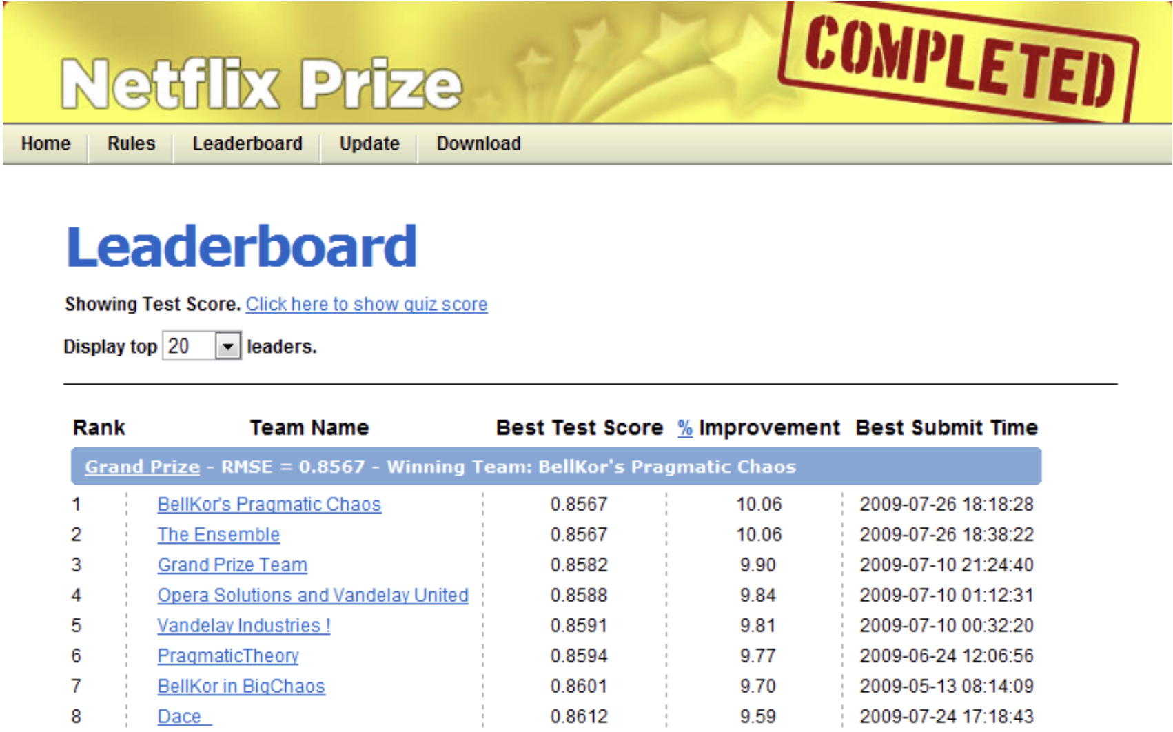
• 100M ratings from ~0.5M users on ~18k movies.

• Grand prize was $1M for the first team to reduce squared error at least by 10%.

• Winning entry (and most entries) used collaborative filtering:

• A simple collaborative filtering method that does really well:

  • “Regularized matrix factorization”. Now adopted by many companies.

4.1 Intuition

• People who agreed in the past are likely to agree again in future.

• We may have similar users and similar items which can help us predict missing entries.

• Leverage social information to provide recommendations.

• Given a utility matrix with many missing entries, how can we predict missing ratings?

\[\begin{split} \begin{bmatrix} ? & ? & \checkmark & ? & \checkmark\\ \checkmark & ? & ? & ? & ?\\ ? & \checkmark & \checkmark & ? & \checkmark\\ ? & ? & ? & ? & ?\\ ? & ? & ? & \checkmark & ?\\ ? & \checkmark & \checkmark & ? & \checkmark \end{bmatrix} \end{split}\]

Can we use something like PCA?

• We are not exactly interested in individual ratings or clicks. We want to find users with similar tastes.

• So we want to learn some latent features related to typical users and typical items.

• We have used PCA/LSA to extract meaningful features before.

• Can we use the same idea here? Yes!

• Collaborative filtering main idea

  • Run PCA-like algorithm on the utility matrix to learn latent features related to typical users and typical items.

  • Use reconstructions to fill in missing entries.

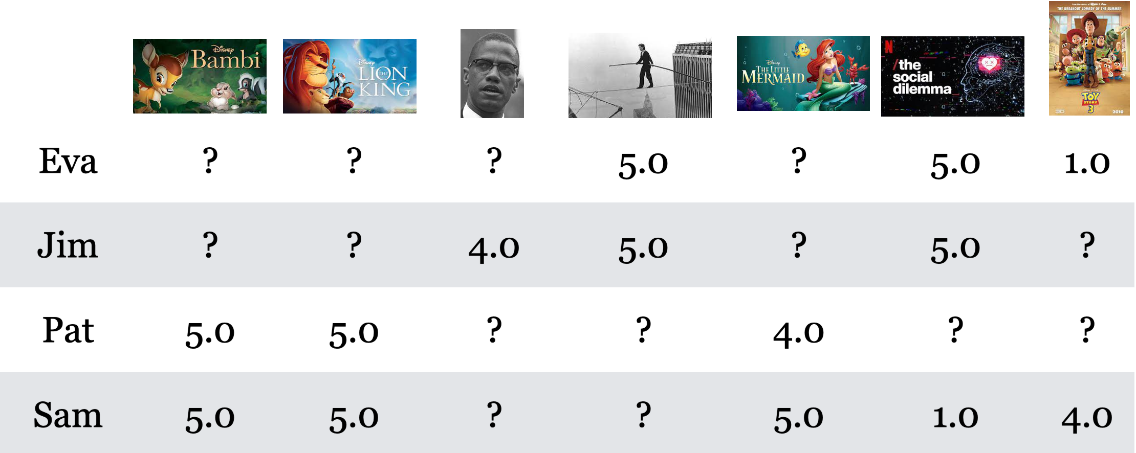
4.2 Toy movie recommendation example

• Let’s walk through our movie recommendation toy example.

• The toy data below contains movie ratings for seven movies given by 4 users.

• Do you see any pattern here?

• In this toy example, we see clear groups of movies and users.

  • For movies: Children movies and documentaries

  • For users: Children movie lovers and documentary lovers

• How can we identify such latent features?

  • Can we use something similar to PCA or LSA (TruncatedSVD)?
    
    

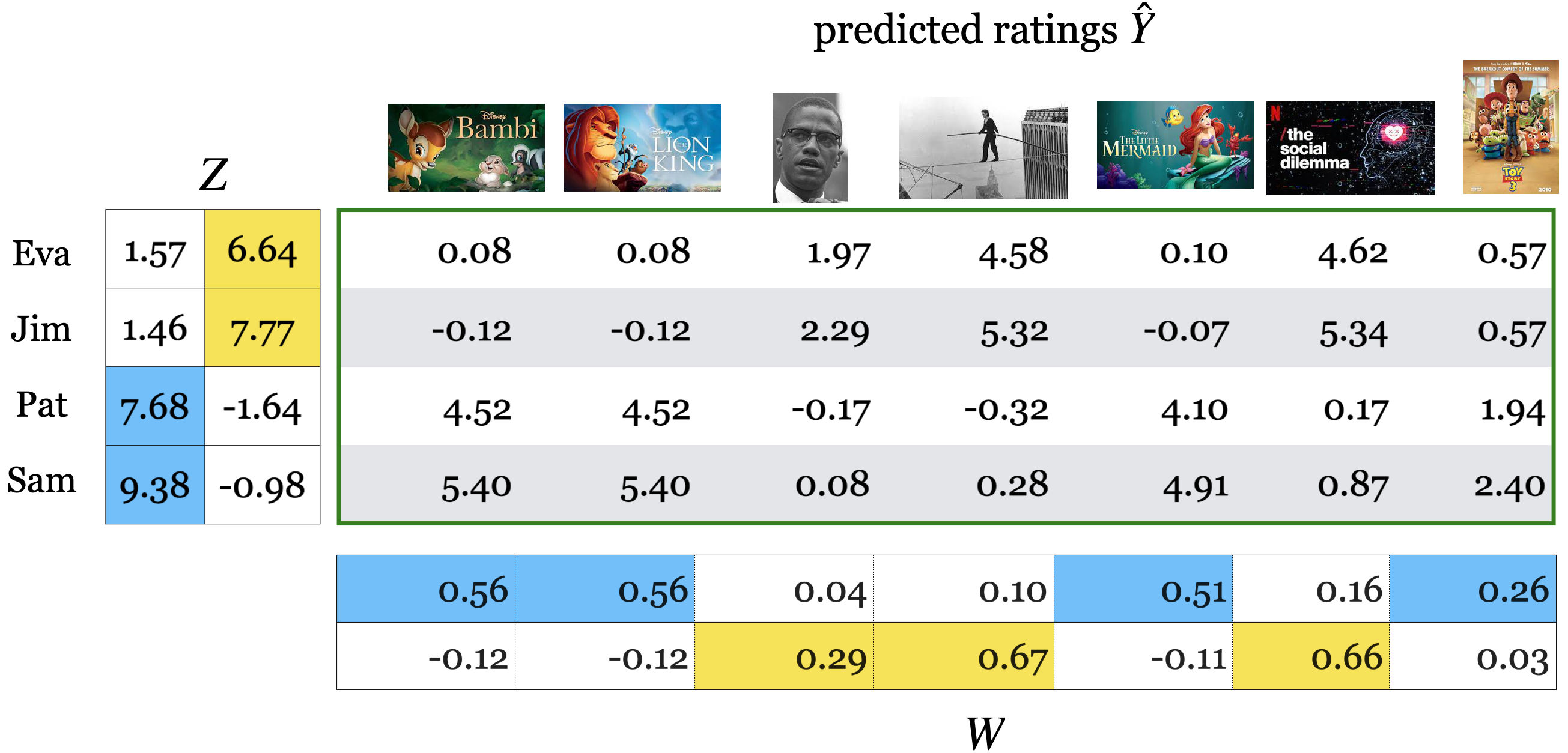
• Once we identify latent features with TruncatedSVD we can get \(Z\) and \(W\) and we can fill in the missing entries by reconstructing the matrix with the product \(Z@W\).

• \(Z\) has embeddings or representations of users and \(W\) has embeddings of items.

• The rating prediction for a user-item pair is the dot product between the embedding of the user and embedding of the item.

• With this approach it’s possible to get some rating predictions which are smaller than zero or greater than 5.

Let’s try this out.

toy_ratings = pd.read_csv(DATA_DIR + "toy-movie-ratings.csv")
toy_ratings

	user_id	movie_id	rating
0	Sam	Lion King	5
1	Sam	Toy Story	4
2	Sam	The Little Mermaid	5
3	Sam	Bambi	5
4	Sam	The Social Dilemma	1
5	Eva	Toy Story	1
6	Eva	The Social Dilemma	5
7	Eva	Man on Wire	5
8	Pat	The Little Mermaid	4
9	Pat	Lion King	5
10	Pat	Bambi	5
11	Jim	The Social Dilemma	5
12	Jim	Malcolm x	4
13	Jim	Man on Wire	5

Let’s create the utility matrix.

N_toy = len(np.unique(toy_ratings["user_id"]))
M_toy = len(np.unique(toy_ratings["movie_id"]))
print(f"Number of users (N)  : {N_toy}")
print(f"Number of movies (M) : {M_toy}")

Number of users (N)  : 4
Number of movies (M) : 7

user_mapper_toy = dict(zip(np.unique(toy_ratings["user_id"]), list(range(N_toy))))
item_mapper_toy = dict(zip(np.unique(toy_ratings["movie_id"]), list(range(M_toy))))
user_inverse_mapper_toy = dict(
    zip(list(range(N_toy)), np.unique(toy_ratings["user_id"]))
)
item_inverse_mapper_toy = dict(
    zip(list(range(M_toy)), np.unique(toy_ratings["movie_id"]))
)

Y_toy = create_Y_from_ratings(
    toy_ratings, N_toy, M_toy, user_mapper_toy, item_mapper_toy, user_key="user_id", item_key="movie_id"
)
utility_mat_toy = pd.DataFrame(
    Y_toy, columns=item_mapper_toy.keys(), index=user_mapper_toy.keys()
)
utility_mat_toy

	Bambi	Lion King	Malcolm x	Man on Wire	The Little Mermaid	The Social Dilemma	Toy Story
Eva	NaN	NaN	NaN	5.0	NaN	5.0	1.0
Jim	NaN	NaN	4.0	5.0	NaN	5.0	NaN
Pat	5.0	5.0	NaN	NaN	4.0	NaN	NaN
Sam	5.0	5.0	NaN	NaN	5.0	1.0	4.0

from sklearn.decomposition import PCA, TruncatedSVD

data_toy = utility_mat_toy.to_numpy()
model_toy = TruncatedSVD(n_components=2, random_state=42)

# model_toy.fit(data_toy) # This won't work.

• We have missing data and we need to impute it to some numeric values so that we can train TruncatedSVD on it.

• How about replacing missing data with zeros?

data_svd_toy = np.nan_to_num(data_toy)  # replace all nan values with zeros
model_toy = TruncatedSVD(n_components=2, random_state=42)
model_toy.fit(data_svd_toy);

Understanding the Transformed Data \(Z\)

• \(Z\) represents users in terms of latent features rather than raw movie ratings.

• Each row in \(Z\) corresponds to a user, where the values capture their preferences for different latent features of movies.

• In this case, we can interpret the two latent features as “Children’s Movies” and “Documentaries”.

• Users with high values in the first column prefer children’s movies.

• Users with high values in the second column prefer documentaries.

Z_toy = model_toy.transform(data_svd_toy)
Z_df = pd.DataFrame(
    Z_toy, index=user_mapper_toy.keys(), columns=["Children's movies??", "Documentaries??"]
)
Z_df.round(2)

	Children's movies??	Documentaries??
Eva	1.57	6.64
Jim	1.46	7.77
Pat	7.68	-1.64
Sam	9.38	-0.98

Understanding \(W\)

• \(W\) represents items (movies) in terms of latent features.

• Each column in \(W\) indicates how strongly a latent feature is associated with different movies.

• Just like with \(Z\), we can interpret the latent factors in \(W\) as “Children’s Movies” and “Documentaries”.

• Movies with high values in the first row align more with children’s movies.

• Movies with high values in the second row align more with documentaries.

W_toy = model_toy.components_

W_df = pd.DataFrame(
    W_toy,
    columns=item_mapper_toy.keys(),
    index=["Children's movies??", "Documentaries??"],
)
W_df.round(2)

	Bambi	Lion King	Malcolm x	Man on Wire	The Little Mermaid	The Social Dilemma	Toy Story
Children's movies??	0.56	0.56	0.04	0.10	0.51	0.16	0.26
Documentaries??	-0.12	-0.12	0.29	0.67	-0.11	0.66	0.03

In recommendation systems, items are features of users and users are features of items. So we can also think of \(W\) as representation of each movie in terms of latent features of users.

W_df.T

	Children's movies??	Documentaries??
Bambi	0.562779	-0.121174
Lion King	0.562779	-0.121174
Malcolm x	0.038657	0.287367
Man on Wire	0.100051	0.666422
The Little Mermaid	0.512129	-0.106044
The Social Dilemma	0.161957	0.657316
Toy Story	0.257970	0.025021

How Do We Get the Predicted Ratings?

• The predicted rating \(\hat{Y}\) for a user and a movie is obtained by computing the dot product of the user’s latent feature vector (row in \(Z\)) and the movie’s latent feature vector (column in \(W\)).

• This measures how well the user’s preferences align with the movie’s characteristics.

pd.DataFrame(Z_toy@W_toy).round(2)

	0	1	2	3	4	5	6
0	0.08	0.08	1.97	4.58	0.10	4.62	0.57
1	-0.12	-0.12	2.29	5.32	-0.07	5.34	0.57
2	4.52	4.52	-0.17	-0.32	4.10	0.17	1.94
3	5.40	5.40	0.08	0.28	4.91	0.87	2.40

4.3 Interpretation of \(Z\) and \(W\) in collaborative filtering

• Given a utility matrix \(Y\) and a specified number of components \(k\) (representing the number of latent features), PCA decomposes the utility matrix \(Y\) into two matrices, \(Z\) and \(W\), as shown below.

\[Y_{N \times M} \approx Z_{N \times k} W_{k \times M}\]

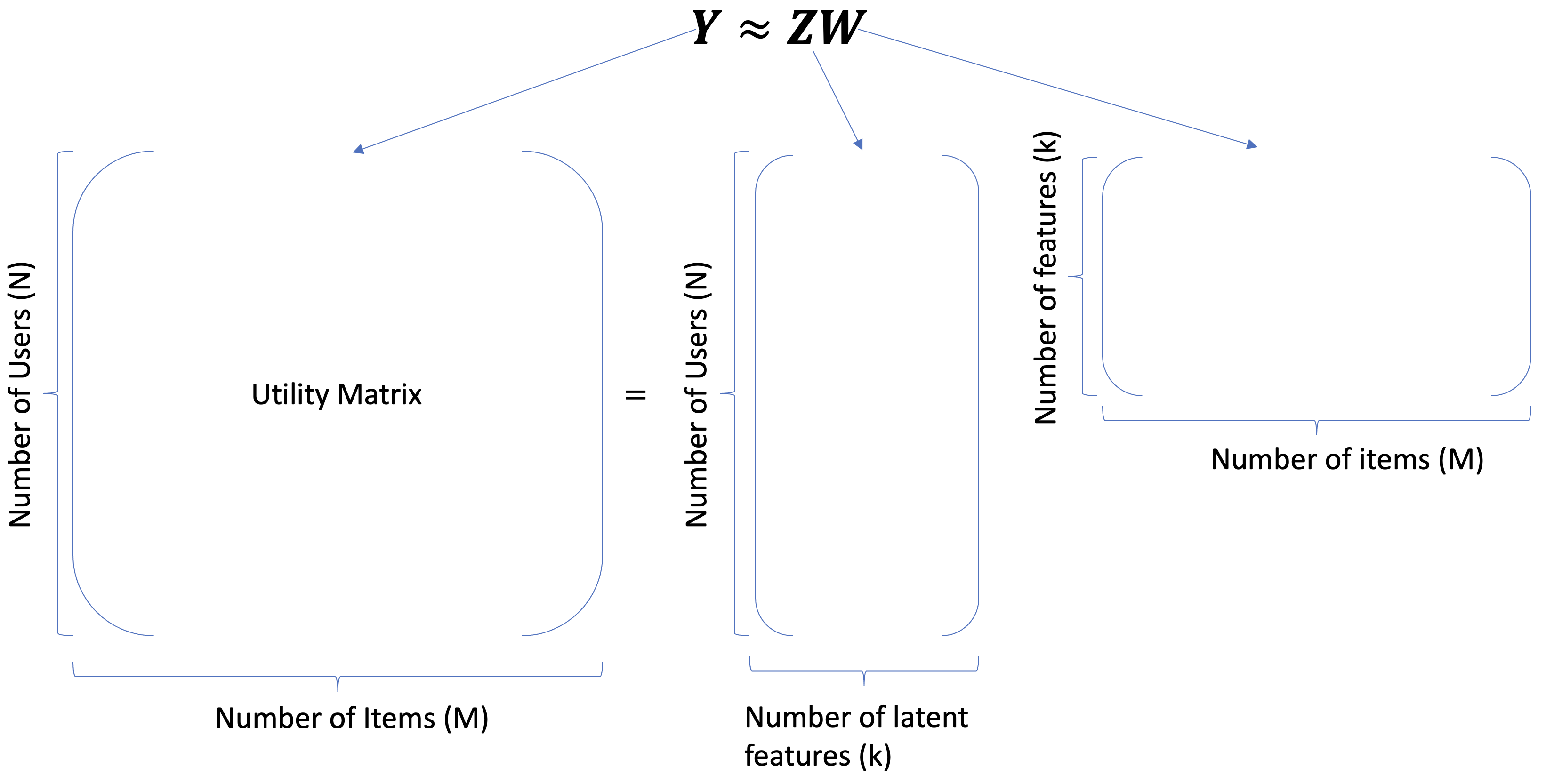
In this context, while the mathematical model remains consistent, the interpretation of the output differs significantly from traditional PCA applications.

• In standard PCA, we maintain a clear distinction between features and examples:

  • \(Z\) is viewed as the matrix representing transformed examples (data points in the new space).

  • \(W\) consists of basis vectors that define the new feature space.

• In recommendation systems, however, this distinction becomes less rigid:

  • Users can be seen as “features” from the perspective of items.

  • Similarly, items can be seen as “features” from the perspective of users.

• The matrix \(Z\) effectively maps users to latent item features, where:

  • Each row in \(Z\) represents a user profile in terms of latent item preferences.

• Conversely, \(W\) maps items to latent user features, where:

  • Each column in \(W\) represents an item profile in terms of latent user preferences.

4.4 Loss function of collaborative filtering

Can we use the loss function of PCA for this?

\[f(Z, W) = \sum_{i=1}^{n} \lVert{W^Tz_i - y_i}\rVert^2_2 \]

• \(W^Tz_i \rightarrow\) reconstructed rating

• \(y_i \rightarrow\) original rating

• Here, the problem with using conventional SVD is that

  • We have many missing entries

  • SVD is undefined when the matrix has missing entries.

Possible solutions

• How about applying some imputation of the missing values?

  • Inaccurate imputation might distort the data

  • The loss function will be dominated by large number of entries which are not part of the real data

• How about summing over only the available ratings in \(R\)?

  • Prone to overfitting
    $\(f(Z, W) = \sum_{(i,j) \in R} ((w_j^Tz_i) - y_{ij})^2\)$

A typical loss function for recommendation systems

• Consider only observed ratings and add regularization to avoid overfitting.

• Here we are adding L2 regularization to penalize weights in \(W\) and \(Z\).

\[f(Z, W) = \sum_{(i,j) \in R} ((w_j^Tz_i) - y_{ij})^2 + \frac{\lambda_1}{2}\lVert Z \lVert_2^2 + \frac{\lambda_2}{2}\lVert W \lVert_2^2\]

• This regularized SVD gave 7% improvement on the Netflix problem!

(Optional) Optimization

Two algorithms are commonly used to minimize this objective function:

• Stochastic gradient descent (SGD)

• Weighted Alternating Least Squares (WALS) is specialized to this particular loss function

  • Allows for massive parallelization

  • Preferred when the data is implicit data and not sparse

(Optional) Adding Global/User/Item biases

• Our standard latent-factor model gives reconstructions for entries in matrix \(Y\) as

\[\hat{y}_{ij} = w^T_jz_i\]

• Sometimes we don’t assume the \(y_{ij}\) has a mean of zero.

• We could add bias \(\beta\) reflecting average overall rating:

\[\hat{y}_{ij} = \beta + w^T_jz_i\]

• We could also add user-specific bias \(\beta_i\) and item-specific bias \(\beta_j\)

\[\hat{y}_{ij} = \beta + \beta_i + \beta_j + w^T_jz_i\]

• Some users rate things higher on average and some movies are rated higher on average.

• The bias terms can also be regularized.

4.5 surprise package for rating prediction

• Since our loss function is slightly different, we cannot really use PCA or LSA implementations in scikit-learn.

• We’ll be using a package called Surprise.

pip install scikit-surprise

• This package implements the famous SVD algorithm popularized during Netflix Prize.

• The loss function above is minimized using stochastic gradient descent.

Let’s try it out on our toy utility matrix.

import surprise
from surprise import SVD, Dataset, Reader, accuracy

Let’s predict ratings with collaborative filtering.

reader = Reader()
data = Dataset.load_from_df(toy_ratings, reader)  # Load the data

trainset, validset = surprise.model_selection.train_test_split(
    data, test_size=0.01, random_state=42
)  # Split the data

k = 2
algo = SVD(n_factors=k, random_state=42)
algo.fit(trainset)
preds = algo.test(trainset.build_testset())
preds

[Prediction(uid='Pat', iid='Lion King', r_ui=5.0, est=4.418103946765089, details={'was_impossible': False}),
 Prediction(uid='Pat', iid='The Little Mermaid', r_ui=4.0, est=4.3238904851989135, details={'was_impossible': False}),
 Prediction(uid='Pat', iid='Bambi', r_ui=5.0, est=4.429962029063298, details={'was_impossible': False}),
 Prediction(uid='Jim', iid='The Social Dilemma', r_ui=5.0, est=4.074699112946736, details={'was_impossible': False}),
 Prediction(uid='Jim', iid='Malcolm x', r_ui=4.0, est=4.2490893833663055, details={'was_impossible': False}),
 Prediction(uid='Jim', iid='Man on Wire', r_ui=5.0, est=4.435013885036921, details={'was_impossible': False}),
 Prediction(uid='Sam', iid='Lion King', r_ui=5.0, est=4.247622025394618, details={'was_impossible': False}),
 Prediction(uid='Sam', iid='The Little Mermaid', r_ui=5.0, est=4.157477218712453, details={'was_impossible': False}),
 Prediction(uid='Sam', iid='Toy Story', r_ui=4.0, est=3.81385601327263, details={'was_impossible': False}),
 Prediction(uid='Sam', iid='The Social Dilemma', r_ui=1.0, est=3.883247434553506, details={'was_impossible': False}),
 Prediction(uid='Sam', iid='Bambi', r_ui=5.0, est=4.245514990652595, details={'was_impossible': False}),
 Prediction(uid='Eva', iid='Toy Story', r_ui=1.0, est=3.6186861930694434, details={'was_impossible': False}),
 Prediction(uid='Eva', iid='Man on Wire', r_ui=5.0, est=4.094092586099001, details={'was_impossible': False})]

from collections import defaultdict

rating_preds = defaultdict(list)
for uid, iid, true_r, est, _ in preds:
    rating_preds[uid].append((iid, est))

rating_preds

defaultdict(list,
            {'Pat': [('Lion King', 4.418103946765089),
              ('The Little Mermaid', 4.3238904851989135),
              ('Bambi', 4.429962029063298)],
             'Jim': [('The Social Dilemma', 4.074699112946736),
              ('Malcolm x', 4.2490893833663055),
              ('Man on Wire', 4.435013885036921)],
             'Sam': [('Lion King', 4.247622025394618),
              ('The Little Mermaid', 4.157477218712453),
              ('Toy Story', 3.81385601327263),
              ('The Social Dilemma', 3.883247434553506),
              ('Bambi', 4.245514990652595)],
             'Eva': [('Toy Story', 3.6186861930694434),
              ('Man on Wire', 4.094092586099001)]})

What’s the validation RMSE?

svd_preds = algo.test(validset)
accuracy.rmse(svd_preds, verbose=True)

RMSE: 1.2666

1.266552791944334

Cross-validation for recommender systems

• We can also carry out cross-validation and grid search with this package.

• Let’s look at an example of cross-validation.

from surprise.model_selection import cross_validate

pd.DataFrame(cross_validate(algo, data, measures=["RMSE", "MAE"], cv=3, verbose=True))

Evaluating RMSE, MAE of algorithm SVD on 3 split(s).

                  Fold 1  Fold 2  Fold 3  Mean    Std     
RMSE (testset)    1.5955  1.0672  1.8088  1.4905  0.3118  
MAE (testset)     1.1333  0.9562  1.1730  1.0875  0.0943  
Fit time          0.00    0.00    0.00    0.00    0.00    
Test time         0.00    0.00    0.00    0.00    0.00    

	test_rmse	test_mae	fit_time	test_time
0	1.595506	1.133279	0.000259	0.000032
1	1.067154	0.956203	0.000259	0.000020
2	1.808816	1.173038	0.000347	0.000019

❓❓ Questions for you

Exercise 7.2 Select all of the following statements which are True (iClicker)

• (A) Collaborative filtering is a technique used to make recommendations based on the preferences of similar users or items.

• (B) The primary difference between PCA and collaborative filtering is that the loss function in the latter only includes the available ratings and regularization terms.

• (C) When you apply collaborative filtering on movie ratings data with ratings in the range 0 to 5, it’s possible to get a predicted rating outside that range.

• (D) Collaborative filtering might have problems if a new item shows up.

• (E) Collaborative filtering might have problems if a new user shows up.

V’s Solutions!

• A, B, C, D, E

Final comments and summary

Formulating the problem of recommender systems

• We are given ratings data.

• We use this data to create utility matrix which encodes interactions between users and items.

• The utility matrix has many missing entries.

• We defined recommendation systems problem as matrix completion problem.

Collaborative filtering

• Collaborative filtering is an unsupervised approach to recommendation systems.

• Surprisingly we use PCA-like approach.

• We factorize the utility matrix into \(Z\) and \(W\).

• \(Z\) has embeddings for users with latent features of items

• \(W^T\) has embeddings for items with latent features of users

• The key idea is that the loss function only includes the available ratings and regularization terms for \(W\) and \(Z\) to avoid overfitting.

• Be mindful of the consequences recommendation systems.

• Companies such as Amazon, Netflix, Facebook, Google (YouTube), which extensively use recommendation systems, are profit-driven and so they design these systems to maximize user attention; their focus is not necessarily human well-being.

• There are tons of news and research articles on serious consequences of recommendation systems.

• Some weird stories which got media attention

  • How Target Figured Out A Teen Girl Was Pregnant Before Her Father Did

• More serious consequences are in political contexts.

  • Facebook Admits It Was Used to Incite Violence in Myanmar

  • YouTube Extremism and the Long Tail

• Check out this recent article: Users, advertisers – we are all trapped in the ‘enshittification’ of the internet

My advice

• Ask hard and uncomfortable questions to yourself (and to your employer if possible) before implementing and deploying such systems.

Resources

• MATRIX FACTORIZATION TECHNIQUES FOR RECOMMENDER SYSTEMS

• Recommendation Systems chapter from Dive into Deep Learning

• Google developer’s advanced courses

• Collaborative filtering for recommendation systems in Python, by N. Hug

• An interesting talk: The paradox of choice

• How Netflix’s Recommendations System Works

• Hands on Recommendation Systems with Python