Lecture 6: Topic Modeling

Lecture 6: Topic Modeling#

UBC Master of Data Science program, 2024-25

Imports, LO#

Imports#

import os, sys
import numpy as np
import pandas as pd
import matplotlib.pyplot as plt

pd.set_option("display.max_colwidth", 200)

DATA_DIR = os.path.join(os.path.abspath(".."), "data/")
sys.path.append(os.path.join(os.path.abspath(".."), "code"))
from plotting_functions import *

---------------------------------------------------------------------------
ImportError                               Traceback (most recent call last)
Cell In[1], line 10
      8 DATA_DIR = os.path.join(os.path.abspath(".."), "data/")
      9 sys.path.append(os.path.join(os.path.abspath(".."), "code"))
---> 10 from plotting_functions import *

File ~/MDS/2024-25/563/DSCI_563_unsup-learn/lectures/code/plotting_functions.py:7
      5 import matplotlib.pyplot as plt
      6 from matplotlib.colors import ListedColormap, colorConverter, LinearSegmentedColormap
----> 7 from scipy.spatial import distance
      8 from sklearn.metrics import euclidean_distances
      9 from sklearn.manifold import MDS

File ~/miniforge3/envs/jbook/lib/python3.12/site-packages/scipy/spatial/__init__.py:110
      1 """
      2 =============================================================
      3 Spatial algorithms and data structures (:mod:`scipy.spatial`)
   (...)
    107    QhullError
    108 """  # noqa: E501
--> 110 from ._kdtree import *
    111 from ._ckdtree import *  # type: ignore[import-not-found]
    112 from ._qhull import *

File ~/miniforge3/envs/jbook/lib/python3.12/site-packages/scipy/spatial/_kdtree.py:4
      1 # Copyright Anne M. Archibald 2008
      2 # Released under the scipy license
      3 import numpy as np
----> 4 from ._ckdtree import cKDTree, cKDTreeNode  # type: ignore[import-not-found]
      6 __all__ = ['minkowski_distance_p', 'minkowski_distance',
      7            'distance_matrix',
      8            'Rectangle', 'KDTree']
     11 def minkowski_distance_p(x, y, p=2):

File _ckdtree.pyx:11, in init scipy.spatial._ckdtree()

File ~/miniforge3/envs/jbook/lib/python3.12/site-packages/scipy/sparse/__init__.py:315
    312 from ._sputils import get_index_dtype, safely_cast_index_arrays
    314 # For backward compatibility with v0.19.
--> 315 from . import csgraph
    317 # Deprecated namespaces, to be removed in v2.0.0
    318 from . import (
    319     base, bsr, compressed, construct, coo, csc, csr, data, dia, dok, extract,
    320     lil, sparsetools, sputils
    321 )

File ~/miniforge3/envs/jbook/lib/python3.12/site-packages/scipy/sparse/csgraph/__init__.py:187
    158 __docformat__ = "restructuredtext en"
    160 __all__ = ['connected_components',
    161            'laplacian',
    162            'shortest_path',
   (...)
    184            'csgraph_to_masked',
    185            'NegativeCycleError']
--> 187 from ._laplacian import laplacian
    188 from ._shortest_path import (
    189     shortest_path, floyd_warshall, dijkstra, bellman_ford, johnson, yen,
    190     NegativeCycleError
    191 )
    192 from ._traversal import (
    193     breadth_first_order, depth_first_order, breadth_first_tree,
    194     depth_first_tree, connected_components
    195 )

File ~/miniforge3/envs/jbook/lib/python3.12/site-packages/scipy/sparse/csgraph/_laplacian.py:7
      5 import numpy as np
      6 from scipy.sparse import issparse
----> 7 from scipy.sparse.linalg import LinearOperator
      8 from scipy.sparse._sputils import convert_pydata_sparse_to_scipy, is_pydata_spmatrix
     11 ###############################################################################
     12 # Graph laplacian

File ~/miniforge3/envs/jbook/lib/python3.12/site-packages/scipy/sparse/linalg/__init__.py:129
      1 """
      2 Sparse linear algebra (:mod:`scipy.sparse.linalg`)
      3 ==================================================
   (...)
    126 
    127 """
--> 129 from ._isolve import *
    130 from ._dsolve import *
    131 from ._interface import *

File ~/miniforge3/envs/jbook/lib/python3.12/site-packages/scipy/sparse/linalg/_isolve/__init__.py:4
      1 "Iterative Solvers for Sparse Linear Systems"
      3 #from info import __doc__
----> 4 from .iterative import *
      5 from .minres import minres
      6 from .lgmres import lgmres

File ~/miniforge3/envs/jbook/lib/python3.12/site-packages/scipy/sparse/linalg/_isolve/iterative.py:5
      3 from scipy.sparse.linalg._interface import LinearOperator
      4 from .utils import make_system
----> 5 from scipy.linalg import get_lapack_funcs
      7 __all__ = ['bicg', 'bicgstab', 'cg', 'cgs', 'gmres', 'qmr']
     10 def _get_atol_rtol(name, b_norm, atol=0., rtol=1e-5):

File ~/miniforge3/envs/jbook/lib/python3.12/site-packages/scipy/linalg/__init__.py:203
      1 """
      2 ====================================
      3 Linear algebra (:mod:`scipy.linalg`)
   (...)
    200 
    201 """  # noqa: E501
--> 203 from ._misc import *
    204 from ._cythonized_array_utils import *
    205 from ._basic import *

File ~/miniforge3/envs/jbook/lib/python3.12/site-packages/scipy/linalg/_misc.py:3
      1 import numpy as np
      2 from numpy.linalg import LinAlgError
----> 3 from .blas import get_blas_funcs
      4 from .lapack import get_lapack_funcs
      6 __all__ = ['LinAlgError', 'LinAlgWarning', 'norm']

File ~/miniforge3/envs/jbook/lib/python3.12/site-packages/scipy/linalg/blas.py:213
    210 import numpy as np
    211 import functools
--> 213 from scipy.linalg import _fblas
    214 try:
    215     from scipy.linalg import _cblas

ImportError: dlopen(/Users/kvarada/miniforge3/envs/jbook/lib/python3.12/site-packages/scipy/linalg/_fblas.cpython-312-darwin.so, 0x0002): Library not loaded: @rpath/libgfortran.5.dylib
  Referenced from: <0B9C315B-A1DD-3527-88DB-4B90531D343F> /Users/kvarada/miniforge3/envs/jbook/lib/libopenblas.0.dylib
  Reason: tried: '/Users/kvarada/miniforge3/envs/jbook/lib/libgfortran.5.dylib' (duplicate LC_RPATH '@loader_path'), '/Users/kvarada/miniforge3/envs/jbook/lib/libgfortran.5.dylib' (duplicate LC_RPATH '@loader_path'), '/Users/kvarada/miniforge3/envs/jbook/lib/python3.12/site-packages/scipy/linalg/../../../../libgfortran.5.dylib' (duplicate LC_RPATH '@loader_path'), '/Users/kvarada/miniforge3/envs/jbook/lib/python3.12/site-packages/scipy/linalg/../../../../libgfortran.5.dylib' (duplicate LC_RPATH '@loader_path'), '/Users/kvarada/miniforge3/envs/jbook/bin/../lib/libgfortran.5.dylib' (duplicate LC_RPATH '@loader_path'), '/Users/kvarada/miniforge3/envs/jbook/bin/../lib/libgfortran.5.dylib' (duplicate LC_RPATH '@loader_path'), '/usr/local/lib/libgfortran.5.dylib' (no such file), '/usr/lib/libgfortran.5.dylib' (no such file, not in dyld cache)

import warnings

warnings.filterwarnings("ignore", category=DeprecationWarning)

Learning outcomes#

From this lesson you will be able to

Explain the general idea of topic modeling.
Identify and name the two main approaches for topic modeling.
Describe the key differences between Latent Semantic Analysis (LSA) and Latent Dirichlet Allocation (LDA).
Outline the process of data generation within an LDA topic model.
Explain the process of updating topic assignments in the LDA model at a high level.
Explain the importance of preprocessing in topic modeling.
Carry out topic modeling with sklearn as well as gensim.
Visualize the topics extracted through topic modeling.
Interpret the output of topic modeling.
Name a few possible ways to evaluate a topic model.
Use coherence scores as a guiding tool to choose the number of topics.
Use Top2Vec package for topic modeling.

1. Why topic modeling?#

1.1 Topic modeling motivation#

Topic modeling introduction activity (~5 mins)

Consider the following documents.

toy_df = pd.read_csv(DATA_DIR + "toy_clustering.csv")
toy_df

	text
0	famous fashion model
1	elegant fashion model
2	fashion model at famous probabilistic topic model conference
3	fresh elegant fashion model
4	famous elegant fashion model
5	probabilistic conference
6	creative probabilistic model
7	model diet apple kiwi nutrition
8	probabilistic model
9	kiwi health nutrition
10	fresh apple kiwi health diet
11	health nutrition
12	fresh apple kiwi juice nutrition
13	probabilistic topic model conference
14	probabilistic topi model

Discuss the following questions with your neighbour and write your answers in this Google doc.

Suppose you are asked to identify topics discussed in these documents manually. How many topics would you identify?
What are the prominent words associated with each topic?
Are there documents which are a mixture of multiple topics?

Humans are pretty good at reading and understanding a document and answering questions such as
- What is it about?
- Which documents is it related to?
What if you’re given a large collection of documents on a variety of topics.

Example: A corpus of news articles

Example: A corpus of food magazines

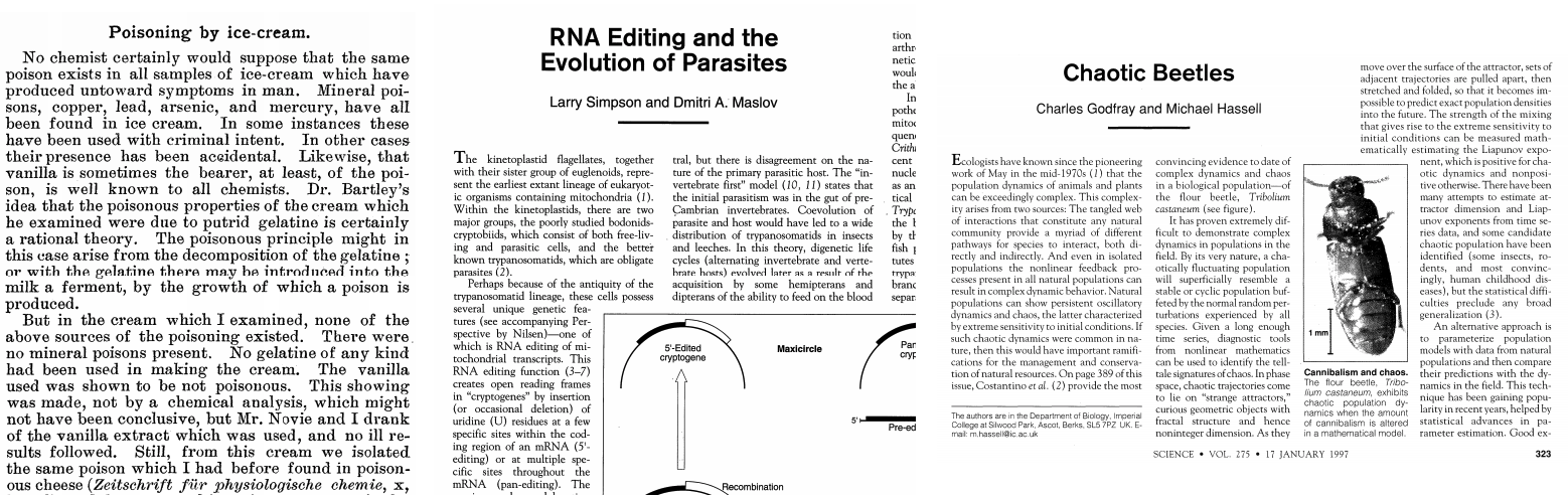
A corpus of scientific articles

(Credit: Dave Blei’s presentation)

It would take years to read all documents and organize and categorize them so that they are easy to search.
You need an automated way
- to get an idea of what’s going on in the data or
- to pull documents related to a certain topic
Topic modeling gives you an ability to summarize the major themes in a large collection of documents (corpus).
- Example: The major themes in a collection of news articles could be
  - politics
  - entertainment
  - sports
  - technology
  - …

Topic modeling is a great EDA tool to get a sense of what’s going on in a large corpus.
Some examples
- If you want to pull documents related to a particular lawsuit.
- You want to examine people’s sentiment towards a particular candidate and/or political party and so you want to pull tweets or Facebook posts related to election.

1.2 How do you do topic modeling?#

A common tool to solve such problems is unsupervised ML methods.
Given the hyperparameter $K$, the goal of topic modeling is to describe a set of documents using $K$ “topics”.
In unsupervised setting, the input of topic modeling is
- A large collection of documents
- A value for the hyperparameter $K$ (e.g., $K = 3$)
and the output is
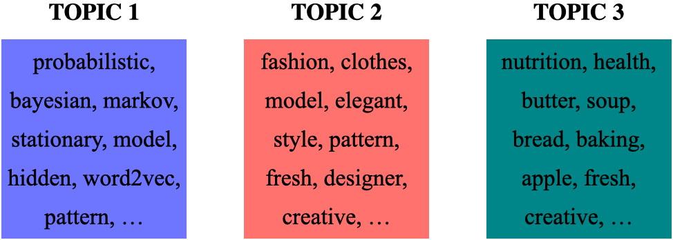
1. Topic-words association
  - For each topic, what words describe that topic?
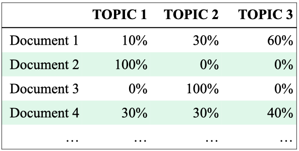
2. Document-topics association
  - For each document, what topics are expressed by the document?

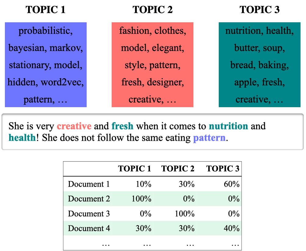
Topic modeling: example 1

Topic-words association
- For each topic, what words describe that topic?
- A topic is a mixture of words.

Document-topics association
- For each document, what topics are expressed by the document?
- A document is a mixture of topics.

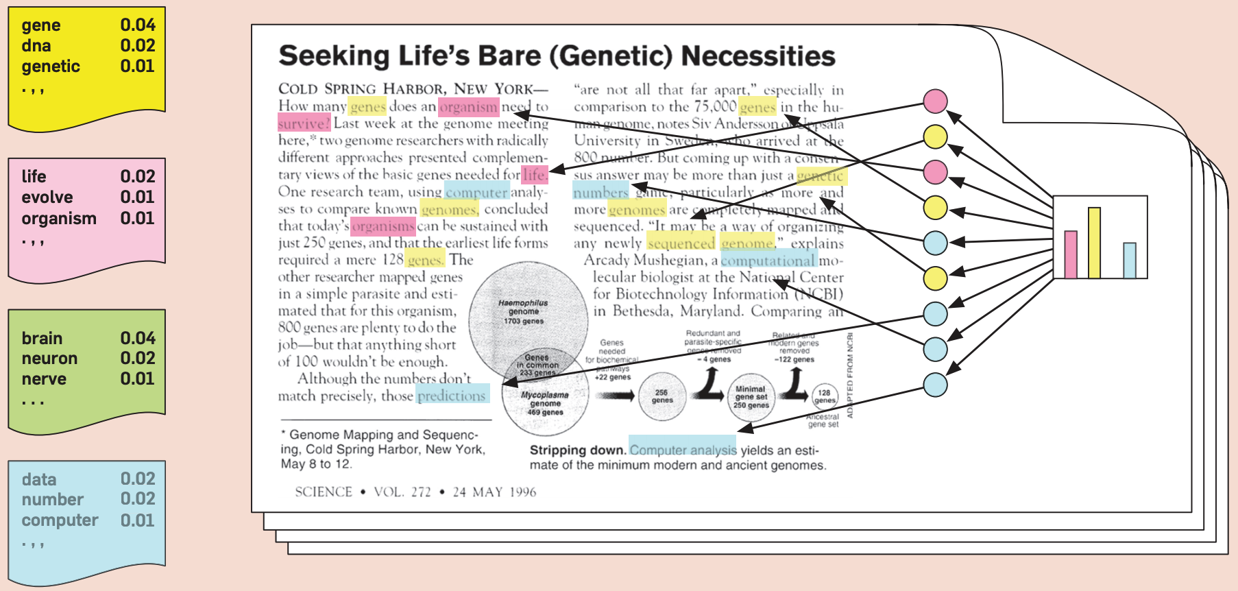
Topic modeling example 2: Scientific papers

Topic modeling: Input

Credit: David Blei’s presentation

Topic modeling: output

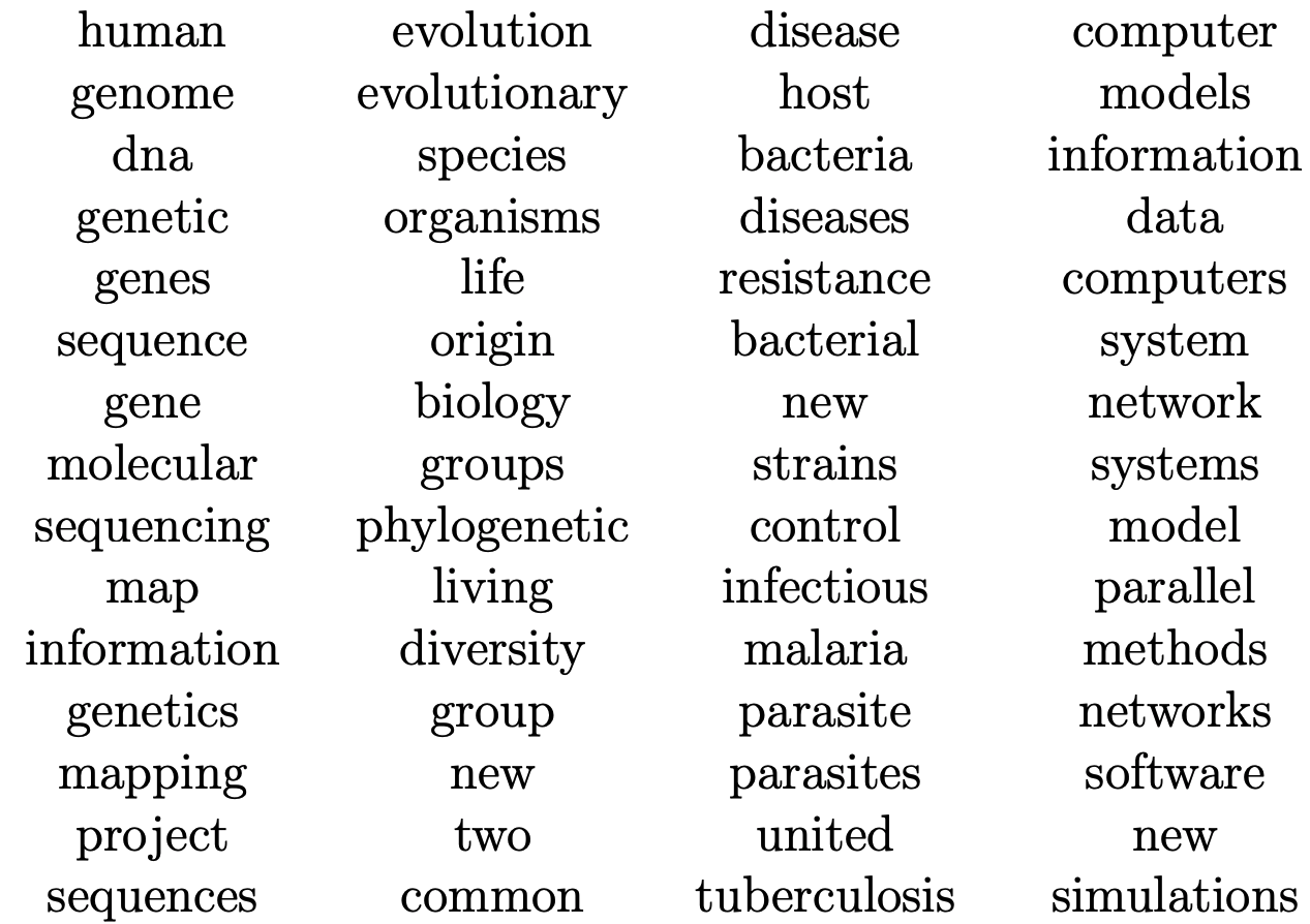
(Credit: David Blei’s presentation)

Assigning labels is a human thing.

(Credit: David Blei’s presentation)

Topic modeling example 3: LDA topics in Yale Law Journal

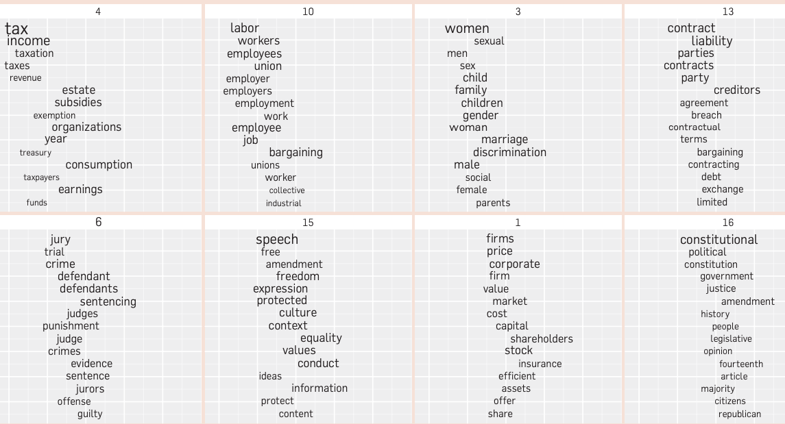
(Credit: David Blei’s paper)

Topic modeling example 3: LDA topics in social media

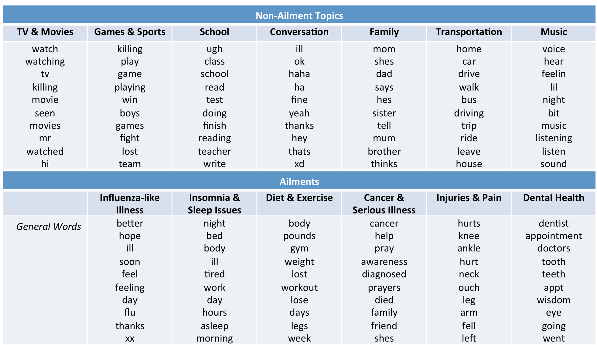
(Credit: Health topics in social media)

Based on the tools in your toolbox what would you use for topic modeling?

There are two main approaches for topic modeling

Topic modeling as matrix factorization (LSA)
Latent Dirichlet Allocation (LDA)

Topic modeling as matrix factorization

We have seen this before in DSCI 563!
You can think of topic modeling as a matrix factorization problem.

\[X_{n \times d} \approx Z_{n \times k}W_{k \times d}\]

Where
- $n \rightarrow $ Number of documents
- $k \rightarrow $ Number of topics
- $d \rightarrow $ Number of features (e.g., the size of vocabulary)
$Z$ gives us document-topic assignments and $W$ gives us topic-word assignments.
This is LSA and we used sklearn’s TruncatedSVD for matrix factorization using SVD (without centering the data).
The idea is to reduce the dimensionality of the data to extract some semantically meaningful components.

Let’s try LSA on the toy dataset above.

toy_df

	text
0	famous fashion model
1	elegant fashion model
2	fashion model at famous probabilistic topic model conference
3	fresh elegant fashion model
4	famous elegant fashion model
5	probabilistic conference
6	creative probabilistic model
7	model diet apple kiwi nutrition
8	probabilistic model
9	kiwi health nutrition
10	fresh apple kiwi health diet
11	health nutrition
12	fresh apple kiwi juice nutrition
13	probabilistic topic model conference
14	probabilistic topi model

Let’s get BOW representation of the documents.

from sklearn.decomposition import TruncatedSVD
from sklearn.feature_extraction.text import CountVectorizer

cv = CountVectorizer(stop_words="english")
bow = cv.fit_transform(toy_df["text"]).toarray()
bow_df = pd.DataFrame(bow, columns=cv.get_feature_names_out(), index=toy_df["text"])
bow_df

	apple	conference	creative	diet	elegant	famous	fashion	fresh	health	juice	kiwi	model	nutrition	probabilistic	topi	topic
text
famous fashion model	0	0	0	0	0	1	1	0	0	0	0	1	0	0	0	0
elegant fashion model	0	0	0	0	1	0	1	0	0	0	0	1	0	0	0	0
fashion model at famous probabilistic topic model conference	0	1	0	0	0	1	1	0	0	0	0	2	0	1	0	1
fresh elegant fashion model	0	0	0	0	1	0	1	1	0	0	0	1	0	0	0	0
famous elegant fashion model	0	0	0	0	1	1	1	0	0	0	0	1	0	0	0	0
probabilistic conference	0	1	0	0	0	0	0	0	0	0	0	0	0	1	0	0
creative probabilistic model	0	0	1	0	0	0	0	0	0	0	0	1	0	1	0	0
model diet apple kiwi nutrition	1	0	0	1	0	0	0	0	0	0	1	1	1	0	0	0
probabilistic model	0	0	0	0	0	0	0	0	0	0	0	1	0	1	0	0
kiwi health nutrition	0	0	0	0	0	0	0	0	1	0	1	0	1	0	0	0
fresh apple kiwi health diet	1	0	0	1	0	0	0	1	1	0	1	0	0	0	0	0
health nutrition	0	0	0	0	0	0	0	0	1	0	0	0	1	0	0	0
fresh apple kiwi juice nutrition	1	0	0	0	0	0	0	1	0	1	1	0	1	0	0	0
probabilistic topic model conference	0	1	0	0	0	0	0	0	0	0	0	1	0	1	0	1
probabilistic topi model	0	0	0	0	0	0	0	0	0	0	0	1	0	1	1	0

Let’s extract latent features from this data.

from sklearn.pipeline import make_pipeline
lsa_pipe = make_pipeline(
    CountVectorizer(stop_words="english"), TruncatedSVD(n_components=3)
)

Z = lsa_pipe.fit_transform(toy_df["text"]);

pd.DataFrame(
    np.round(Z, 4),
    columns=["latent topic 1 ", "latent topic 2", "latent topic 3"],
    index=toy_df["text"],
)

	latent topic 1	latent topic 2	latent topic 3
text
famous fashion model	1.3395	-0.1852	-0.7211
elegant fashion model	1.2732	-0.1242	-0.9512
fashion model at famous probabilistic topic model conference	2.8280	-0.5133	0.3490
fresh elegant fashion model	1.3594	0.1891	-1.0901
famous elegant fashion model	1.5187	-0.1957	-1.1627
probabilistic conference	0.5673	-0.2133	0.8913
creative probabilistic model	1.1405	-0.1919	0.6450
model diet apple kiwi nutrition	1.0110	1.6361	0.1893
probabilistic model	1.0913	-0.1766	0.5561
kiwi health nutrition	0.1729	1.2872	0.1848
fresh apple kiwi health diet	0.3187	1.8663	0.0410
health nutrition	0.0942	0.7554	0.1220
fresh apple kiwi juice nutrition	0.3187	1.8663	0.0410
probabilistic topic model conference	1.4885	-0.3280	1.0701
probabilistic topi model	1.1405	-0.1919	0.6450

Let’s examine the components learned by LSA.

How much variance is covered by the components?

lsa_pipe.named_steps["truncatedsvd"].explained_variance_ratio_.sum()

0.6388605814592396

W = lsa_pipe.named_steps['truncatedsvd'].components_
W

array([[ 0.07117283,  0.21086319,  0.0492425 ,  0.05741109,  0.17923934,
         0.24550644,  0.35917349,  0.0862183 ,  0.02529475,  0.01376174,
         0.07863696,  0.73479234,  0.06894411,  0.35646458,  0.0492425 ,
         0.1863681 ],
       [ 0.42896386, -0.08426254, -0.01533175,  0.27984656, -0.01045014,
        -0.07144379, -0.06625945,  0.31334502,  0.31231756,  0.1491173 ,
         0.53180999, -0.04752051,  0.44304682, -0.12903277, -0.01533175,
        -0.0672201 ],
       [ 0.03739841,  0.31842229,  0.08889624,  0.03174416, -0.441568  ,
        -0.2115269 , -0.49285279, -0.13892801,  0.04793849,  0.00565424,
         0.06287313, -0.01674034,  0.07402841,  0.57285931,  0.08889624,
         0.19558552]])

print("W.shape: {}".format(W.shape))
vocab = lsa_pipe.named_steps['countvectorizer'].get_feature_names_out()

W.shape: (3, 16)

plot_lda_w_vectors(W, ['topic 0', 'topic 1', 'topic 2'], vocab, width=800, height=600)

Let’s print the topics:

W_sorted = np.argsort(W, axis=1)[:, ::-1]

feature_names = np.array(
    lsa_pipe.named_steps["countvectorizer"].get_feature_names_out()
)
print_topics(
    topics=[0, 1, 2], feature_names=feature_names, sorting=W_sorted, n_words=5
)

topic 0       topic 1       topic 2       
--------      --------      --------      
model         kiwi          probabilistic 
fashion       nutrition     conference    
probabilistic apple         topic         
famous        fresh         creative      
conference    health        topi          

Our features are word counts.
LSA has learned useful “concepts” or latent features from word count features.

2. Topic modeling with Latent Dirichlet Allocation (LDA)#

Attribution: Material and presentation in the next slides is adapted from Jordan Boyd-Graber’s excellent material on LDA.

Another common approach to topic modeling
A Bayesian, probabilistic, and generative approach
- Similar to Gaussian Mixture Models (GMMs), you can think of this as a procedure to generate the data
Developed by David Blei and colleagues in 2003.
- One of the most cited papers in the last 20 years.
Produces topics which are more interpretable and distinct from each other.
DISCLAIMER
- We won’t go into the math because it’s a bit involved and we do not have the time.
- My goal is to give you an intuition of the model and show you how to use it to solve topic modeling problems.

Suppose you are asked to create a probabilistic generative story of how our toy data came to be.

toy_df

	text
0	famous fashion model
1	elegant fashion model
2	fashion model at famous probabilistic topic model conference
3	fresh elegant fashion model
4	famous elegant fashion model
5	probabilistic conference
6	creative probabilistic model
7	model diet apple kiwi nutrition
8	probabilistic model
9	kiwi health nutrition
10	fresh apple kiwi health diet
11	health nutrition
12	fresh apple kiwi juice nutrition
13	probabilistic topic model conference
14	probabilistic topi model

2.1 Possible approaches to generate documents#

LDA is a generative model, which means that it comes up with a story that tells us from what distributions our data might have been generated. In other words, our goal is to effectively convey the process of generating observable data (documents, in this case) from hidden or latent variables (topics and their distributions within documents).

Let’s brainstorm some possible ways documents might have been generated.

Let’s assume all documents have $d$ words and word order doesn’t matter.

Approach 1: Single probability distribution over words

We assume there is one fixed probability distribution over all words and each word $w_j$ comes from this distribution.
To generate a document with $d$ words, we sample words directly from this distribution.
Drawback: All documents look more or less the same. We don’t see any clear grouping.
Want: We want the word distribution to depend upon the topic

Approach 2: Each topic has its own distribution

Instead of having one global word distribution, we assume that there are $k$ topics (e.g., fashion, food, machine learning) and each topic has its own probability distribution over words.
To generate a document with $d$ words
- sample a topic $z$ from the mixture of topics
- sample a word $d$ times from topic $z$’s distribution
Drawback: Now the documents are more diverse but each document is entirely about a single topic, which is unrealistic. In reality, a document often mixes multiple topics.

Approach 3: Introducing a topic distribution for each document

Each document isn’t just about one topic – it has a mixture of topics. So, for each document, we introduce a probability distribution over topics.
Let’s introduce a vector $\theta$ of topic proportions associated with each document.
To generate a document with $d$ words given probabilities $\theta$
- sample $d$ topics from $\theta$
- for each sampled topic, sample a word from the topic distribution

Documents now look realistic. This is exactly what Latent Dirichlet Allocation (LDA) models – documents are mixtures of topics, and topics are mixtures of words.

Latent Dirichlet Allocation (LDA)

Where do topic and word distributions come from?
This is where Dirichlet priors come into play.
LDA assumes that both document-topic distributions and topic-word distributions are drawn from Dirichlet priors, which control how mixed or specialized these distributions are.

How to generate a document with $d$ words:

Sample the document’s topic proportions $\theta$ from a Dirichlet prior.
For each of the $d$ words:
- Sample a topic from the document’s topic distribution $\theta$.
- Sample a word from the corresponding topic’s word distribution.

This process ensures that documents have a mixture of topics, and topics are defined by specific word distributions.

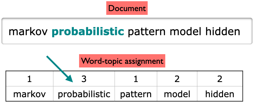
2.2 Generative story of LDA#

The story that tells us how our data was generated.
The generative story of LDA to create Document 1 below:
1. Pick a topic from the topic distribution for Document 1.
2. Pick a word from the selected topic’s word distribution.
Not a realistic story but a mathematically useful story.

Similar to LSA, we fix the number of topics $K$
Topic-word distribution: Each topic is a multinomial distribution over words
Document-topic distribution: Each document is a multinomial distribution over corpus-wide topics

(Credit: David Blei’s presentation)

Topic-word distribution
- If I pick a word from the pink topic, the probability of it being life is 0.02, evolve is 0.01, and organism is 0.01.
- Equivalent to the components $W$ in LSA.
Document-topic distribution
- If I pick a random word from the document, how likely it’s going to be from yellow topic vs. pink topic vs. cyan topic.
- Equivalent to the latent representation $Z$ in LSA.

2.3 LDA inference (high-level)#

Our goal is to infer the underlying distributional structure that explains the observed data.
How can we estimate the following latent variables that characterize the underlying topic structure of the document collection?
- the topic assignments for each word in a given document
- the topic-word distributions
- the document-topic distributions
Typically fit using Bayesian inference
- Most common algorithm is MCMC

Note

(Optional) The Dirichlet distribution is used as a prior distribution in the Bayesian inference process of estimating the topic-word and document-topic distributions because it has some desirable properties such as being a conjugate prior, which means that the posterior has the same form as that of the prior which allows us to compute the posterior distribution of the topic-word and document-topic distributions, given the observed data (i.e., the words in the documents) analytically in closed form, which simplifies the inference process.

How do we find the posterior distribution?

We are interested in the posterior distribution, i.e., the updated probability distribution of the topic assignments for each word in the document, given the observed words in the document and the current estimate of the topic proportions for that document
How do we find it?
- Gibbs sampling (very accurate but very slow, appropriate for small datasets)
- Variational inference (faster but less accurate, extension of expectation maximization, appropriate for medium to large datasets)
Next let’s look at an intuition of Gibbs sampling for topic modeling.

Main Steps in Gibbs Sampling for LDA

Initialization: Assign each word in each document randomly to a topic. This initial assignment gives us a starting point for our counts in the “word-topic” and “document-topic” count tables.
Update Word-Topic Assignment: For each word in each document, perform the following steps:
- Decrease the counts in our count tables (“word-topic counts” and “document-topic counts”) for the current word and its current topic assignment.
- Calculate the probability of each topic for this word, based on the current state of counts (both the document’s topic distribution and the word’s topic distribution across all documents).
- Sample a new topic for the word based on these probabilities.
- Increase the counts in the count tables to reflect this new topic assignment.
Iterate: Repeat the above step for each word in a pass. Multiple passes are done until the assignments converge, which means the changes in topic assignments between sweeps are minimal or below a certain threshold.

After many passes, we can estimate the document-topic distributions and the topic-word distributions from the count tables. These distributions are our model that tells us the topics present in the documents and the words associated with each topic.

Gibbs sampling example

Suppose the number of topics is $3$ and the topics are numbered $1, 2, 3$
initialization: Randomly assign each word in each document to one of the topics.
- The same word in the vocabulary may have different topic assignments in different instances.

With the current topic assignment, here are the topic counts in our document

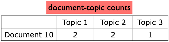
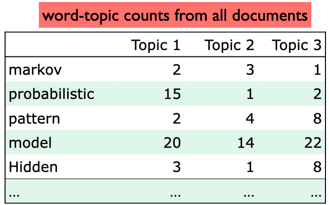
And these are word topic counts in the corpus, i.e., how much each word in the document is liked by each topic.

For each word in our current document (Document 10), calculate how often that word occurs with each topic in all documents.
Note that the counts in the toy example below are made-up counts

How to update Word-Topic Assignment?

Suppose our sampled word-topic assignment is the word probabilistic in Document 10 with assigned topic 3.
Goal: update this word topic assignment.

Step 1: Decrement counts

We want to update the word topic assignment of probabilistic and Topic 3.
How often does Topic 3 occur in Document 10? Once.
How often does the word probabilistic occur with Topic 3 in the corpus? Twice.
Decrement the count of the word from the word-topic counts.

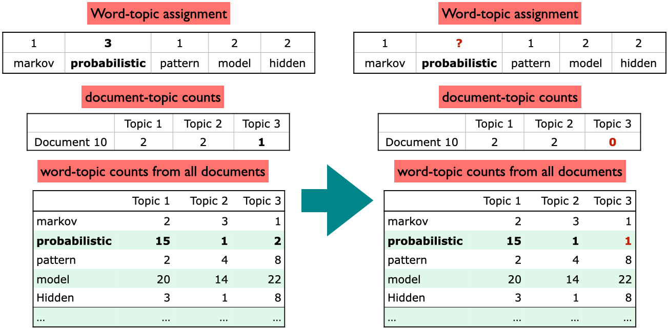
Step 2: Calculating conditional probability distribution

What is the topic preference of Document 10?
What is the preference of the word probabilistic for each topic?

Document 10 likes Topic 1
Topic 1 likes the word probabilistic – it tends to occur a lot in Topic 1.

Step 3: Updating topic assignment

So update the topic of the current word probabilistic in document 10 to topic 1
Update the document-topic and word-topic counts accordingly.

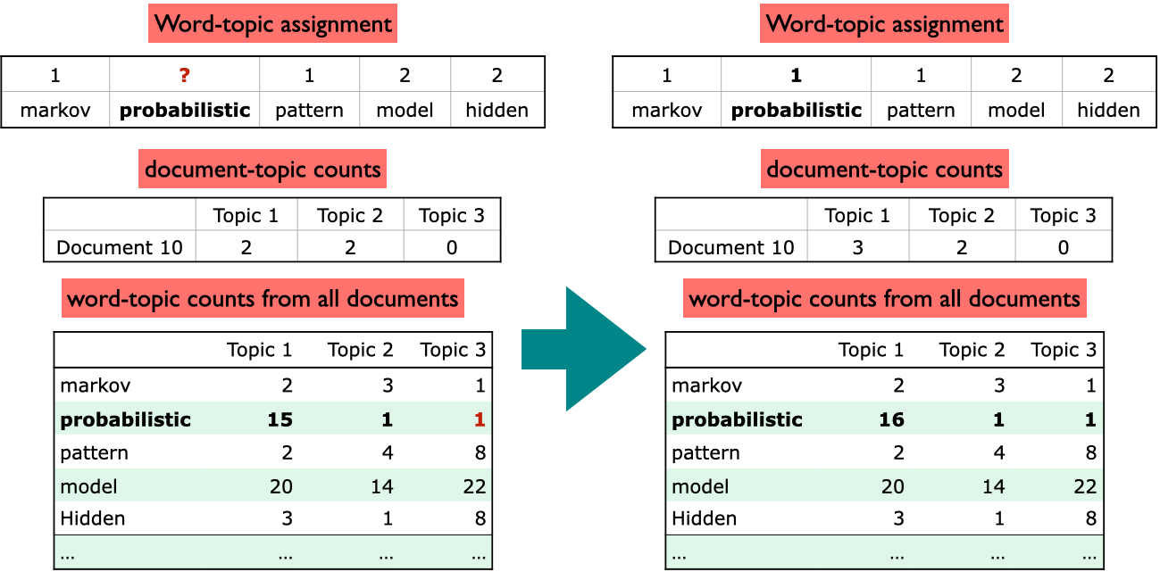
Conclusion

In one pass, the algorithm repeats the above steps for each word in the corpus
If you do this for several passes, meaningful topics emerge.

❓❓ Questions for you#

Exercise: Select all of the following statements which are True (iClicker)#

(A) Latent Dirichlet Allocation (LDA) is an unsupervised approach.
(B) The assumption in topic modeling is that different topics tend to use different words.
(C) We could use LSA for topic modeling, where $Z$ gives us the mixture of topics per document.
(D) In LDA topic model, a document is a mixture of multiple topics.
(E) If I train a topic model on a large collection of news articles with K = 10, I would get 10 topic labels (e.g., sports, culture, politics, finance) as output.

V’s Solutions!

A, B, C, D

Exercise: Questions for class discussion#

What’s the difference between topic modeling and document clustering using algorithms such as K-Means clustering?
Imagine that you are using LSA for topic modeling, where $X$ is bag-of-words representation of $N$ documents and $V$ features (number of words in the vocabulary). Explain which matrix would give you word distribution over topics and which matrix would give you topic distribution over documents. $$X_{N \times V} = Z_{N \times K} W_{K \times V}$$

V’s Solutions!

In clustering with K-Means, documents are grouped based on a similarity measure, and each document is assigned to a single cluster. In contrast, topic modeling produces distributions over words for each topic, as well as distributions over topics per document. Topic modeling can be thought of as a form of soft clustering, where documents are assigned to multiple topics based on their probability distributions rather than a single cluster.
$Z$ would give distribution over topics per document and $W$ would give distribution over words per topic.

3. Topic modeling with Python#

3.1 Topic modeling pipeline#

There are three components in topic modeling pipeline.

Preprocess your corpus.
Train LDA using sklearn or Gensim.
Interpret your topics.

Let’s work with a slightly bigger corpus. We’ll extract text from a few Wikipedia articles and apply topic modeling on these texts.

import wikipedia

queries = [
    "Artificial Intelligence",
    "Supervised Machine Learning",
    "Supreme Court of Canada",
    "Peace, Order, and Good Government",
    "Canadian constitutional law",
    "ice hockey",
    "Google company",
    "Google litigation",
]
wiki_dict = {"wiki query": [], "text": []}
for i in range(len(queries)):
    text = wikipedia.page(queries[i]).content
    wiki_dict["text"].append(text)
    print(len(text))
    wiki_dict["wiki query"].append(queries[i])

wiki_df = pd.DataFrame(wiki_dict)
wiki_df

	wiki query	text
0	Artificial Intelligence	Artificial intelligence (AI) refers to the capability of computational systems to perform tasks typically associated with human intelligence, such as learning, reasoning, problem-solving, percepti...
1	Supervised Machine Learning	In machine learning, supervised learning (SL) is a paradigm where a model is trained using input objects (e.g. a vector of predictor variables) and desired output values (also known as a superviso...
2	Supreme Court of Canada	The Supreme Court of Canada (SCC; French: Cour suprême du Canada, CSC) is the highest court in the judicial system of Canada. It comprises nine justices, whose decisions are the ultimate applicati...
3	Peace, Order, and Good Government	In many Commonwealth jurisdictions, the phrase "peace, order, and good government" (POGG) is an expression used in law to express the legitimate objects of legislative powers conferred by statute....
4	Canadian constitutional law	Canadian constitutional law (French: droit constitutionnel du Canada) is the area of Canadian law relating to the interpretation and application of the Constitution of Canada by the courts. All la...
5	ice hockey	Ice hockey (or simply hockey in North America) is a team sport played on ice skates, usually on an ice skating rink with lines and markings specific to the sport. It belongs to a family of sports ...
6	Google company	Google LLC ( , GOO-gəl) is an American multinational corporation and technology company focusing on online advertising, search engine technology, cloud computing, computer software, quantum comput...
7	Google litigation	Google has been involved in multiple lawsuits over issues such as privacy, advertising, intellectual property and various Google services such as Google Books and YouTube. The company's legal depa...

Preprocessing the corpus

Preprocessing is crucial!
Tokenization, converting text to lower case
Removing punctuation and stopwords
Discarding words with length < threshold or word frequency < threshold
Possibly lemmatization: Consider the lemmas instead of inflected forms.
Depending upon your application, restrict to specific part of speech;
- For example, only consider nouns, verbs, and adjectives

We’ll use spaCy for preprocessing.

# !python -m spacy download en_core_web_md

import spacy

nlp = spacy.load("en_core_web_md")

def preprocess_spacy(
    doc,
    min_token_len=2,
    irrelevant_pos=["ADV", "PRON", "CCONJ", "PUNCT", "PART", "DET", "ADP"],
):
    """
    Given text, min_token_len, and irrelevant_pos carry out preprocessing of the text
    and return a preprocessed string.

    Parameters
    -------------
    doc : (spaCy doc object)
        the spacy doc object of the text
    min_token_len : (int)
        min_token_length required
    irrelevant_pos : (list)
        a list of irrelevant pos tags

    Returns
    -------------
    (str) the preprocessed text
    """

    clean_text = []

    for token in doc:
        if (
            token.is_stop == False  # Check if it's not a stopword
            and len(token) > min_token_len  # Check if the word meets minimum threshold
            and token.pos_ not in irrelevant_pos
        ):  # Check if the POS is in the acceptable POS tags
            lemma = token.lemma_  # Take the lemma of the word
            clean_text.append(lemma.lower())
    return " ".join(clean_text)

wiki_df["text_pp"] = [preprocess_spacy(text) for text in nlp.pipe(wiki_df["text"])]

wiki_df

	wiki query	text	text_pp
0	Artificial Intelligence	Artificial intelligence (AI) refers to the capability of computational systems to perform tasks typically associated with human intelligence, such as learning, reasoning, problem-solving, percepti...	artificial intelligence refer capability computational system perform task associate human intelligence learn reasoning problem solving perception decision making field research computer science d...
1	Supervised Machine Learning	In machine learning, supervised learning (SL) is a paradigm where a model is trained using input objects (e.g. a vector of predictor variables) and desired output values (also known as a superviso...	machine learning supervised learning paradigm model train input object vector predictor variable desire output value know supervisory signal human label training process build function map new dat...
2	Supreme Court of Canada	The Supreme Court of Canada (SCC; French: Cour suprême du Canada, CSC) is the highest court in the judicial system of Canada. It comprises nine justices, whose decisions are the ultimate applicati...	supreme court canada scc french cour suprême canada csc high court judicial system canada comprise justice decision ultimate application canadian law grant permission litigant year appeal decision...
3	Peace, Order, and Good Government	In many Commonwealth jurisdictions, the phrase "peace, order, and good government" (POGG) is an expression used in law to express the legitimate objects of legislative powers conferred by statute....	commonwealth jurisdiction phrase peace order good government pogg expression law express legitimate object legislative power confer statute phrase appear imperial acts parliament letters patent co...
4	Canadian constitutional law	Canadian constitutional law (French: droit constitutionnel du Canada) is the area of Canadian law relating to the interpretation and application of the Constitution of Canada by the courts. All la...	canadian constitutional law french droit constitutionnel canada area canadian law relate interpretation application constitution canada court law canada provincial federal conform constitution law...
5	ice hockey	Ice hockey (or simply hockey in North America) is a team sport played on ice skates, usually on an ice skating rink with lines and markings specific to the sport. It belongs to a family of sports ...	ice hockey hockey north america team sport play ice skate ice skate rink line marking specific sport belong family sport call hockey oppose team use ice hockey stick control advance shoot vulcaniz...
6	Google company	Google LLC ( , GOO-gəl) is an American multinational corporation and technology company focusing on online advertising, search engine technology, cloud computing, computer software, quantum comput...	google llc goo gəl american multinational corporation technology company focus online advertising search engine technology cloud computing computer software quantum computing commerce consumer ele...
7	Google litigation	Google has been involved in multiple lawsuits over issues such as privacy, advertising, intellectual property and various Google services such as Google Books and YouTube. The company's legal depa...	google involve multiple lawsuit issue privacy advertising intellectual property google service google books youtube company legal department expand 100 lawyer year business 2014 grow 400 lawyer go...

Training LDA with sklearn

docs = wiki_df["text_pp"]

from sklearn.feature_extraction.text import CountVectorizer

vectorizer = CountVectorizer()
dtm = vectorizer.fit_transform(wiki_df["text_pp"])

from sklearn.decomposition import LatentDirichletAllocation

n_topics = 3
lda = LatentDirichletAllocation(
    n_components=n_topics, learning_method="batch", max_iter=10, random_state=0
)
document_topics = lda.fit_transform(dtm)

print("lda.components_.shape: {}".format(lda.components_.shape))

lda.components_.shape: (3, 5143)

sorting = np.argsort(lda.components_, axis=1)[:, ::-1]
feature_names = np.array(vectorizer.get_feature_names_out())

print_topics(
    topics=range(3),
    feature_names=feature_names,
    sorting=sorting,
    topics_per_chunk=5,
    n_words=10,
)

topic 0       topic 1       topic 2       
--------      --------      --------      
power         court         google        
intelligence  google        hockey        
problem       case          player        
law           displaystyle  team          
machine       justice       ice           
government    algorithm     league        
human         inc           play          
artificial    function      company       
learning      supreme       game          
provincial    learning      puck          

Training LDA with gensim

I’ll also show you how to do topic modeling with gensim, which we used for Word2Vec, because it’s more flexible.

To train an LDA model with gensim, you need

Document-term matrix
Dictionary (vocabulary)
The number of topics ($K$): num_topics
The number of passes: passes

Let’s first create a dictionary using corpora.Dictionary.
It has two useful methods
- token2id gives token to index mapping
- doc2bow creates bag-of-words representation of a given document

import gensim
from gensim.corpora import Dictionary

corpus = [doc.split() for doc in wiki_df["text_pp"].tolist()]
dictionary = Dictionary(corpus)  # Create a vocabulary for the lda model

list(dictionary.token2id.items())[:4]

[('0700', 0), ('1.6', 1), ('100', 2), ('1099', 3)]

pd.DataFrame(
    dictionary.token2id.keys(), index=dictionary.token2id.values(), columns=["Word"]
)

	Word
0	0700
1	1.6
2	100
3	1099
4	127
...	...
5235	window
5236	windows
5237	wiretap
5238	writer
5239	yuan

5240 rows × 1 columns

Now let’s convert our corpus into document-term matrix for LDA using dictionary.doc2bow.
For each document, it stores the frequency of each token in the document in the format (token_id, frequency).

doc_term_matrix = [dictionary.doc2bow(doc) for doc in corpus]
doc_term_matrix[1][:20]

[(75, 4),
 (86, 3),
 (92, 1),
 (97, 3),
 (98, 1),
 (103, 1),
 (104, 1),
 (107, 3),
 (144, 50),
 (151, 1),
 (170, 4),
 (172, 1),
 (190, 1),
 (191, 4),
 (192, 3),
 (208, 1),
 (212, 1),
 (220, 2),
 (229, 2),
 (248, 3)]

Now we are ready to train an LDA model with Gensim!

from gensim.models import LdaModel

num_topics = 3

lda = LdaModel(
    corpus=doc_term_matrix,
    id2word=dictionary,
    num_topics=num_topics,
    random_state=42,
    passes=10,
)

We can examine the topics and topic distribution for a document in our LDA model

lda.print_topics(num_words=5)  # Topics

[(0,
  '0.033*"google" + 0.007*"search" + 0.007*"company" + 0.005*"intelligence" + 0.005*"use"'),
 (1,
  '0.020*"hockey" + 0.013*"player" + 0.013*"court" + 0.013*"ice" + 0.013*"team"'),
 (2,
  '0.015*"\\displaystyle" + 0.011*"algorithm" + 0.009*"function" + 0.009*"learning" + 0.008*"law"')]

print("Document label: ", wiki_df.iloc[1,0])
print("Topic assignment for document: ", lda[doc_term_matrix[7]])  # Topic distribution

Document label:  Supervised Machine Learning
Topic assignment for document:  [(0, 0.9996161)]

topic_assignment = sorted(lda[doc_term_matrix[1]], key=lambda x: x[1], reverse=True)
df = pd.DataFrame(topic_assignment, columns=["topic id", "probability"])
df

	topic id	probability
0	2	0.999526

new_doc = "After the court yesterday lawyers working on Google lawsuits went to a ice hockey game."
pp_new_doc = preprocess_spacy(nlp(new_doc))
pp_new_doc

'court yesterday lawyer work google lawsuit go ice hockey game'

bow_vector = dictionary.doc2bow(pp_new_doc.split())

topic_assignment = sorted(lda[bow_vector], key=lambda x: x[1], reverse=True)
df = pd.DataFrame(topic_assignment, columns=["topic id", "probability"])
df

	topic id	probability
0	1	0.520430
1	0	0.445166
2	2	0.034403

Main hyperparameters:

num_topics or K: The number of requested latent topics to be extracted from the training corpus.
alpha: A-priori belief on document-topic distribution. When you set alpha as a scalar, it applies symmetrically across all topics, meaning each topic has the same prior importance in documents before observing the actual words. In such cases:
- A lower alpha encourages the model to assign fewer topics to each document, leading to a more sparse representation.
- A higher alpha suggests that documents are likely to contain a mixture of more topics.
eta (often referred to as beta in the literature): A-priori belief on topic-word distribution. When you set eta as a scalar, it applies symmetrically across all topics, meaning each topic has the same prior importance in documents before observing the actual words. In such cases:
- A lower eta indicates that each topic is formed by a smaller set of words
- A higher eta allows topics to be more broadly defined by a large set of words

There is also an auto option for both hyperparameters alpha and eta which learns an asymmetric prior from the data. Check the documentation.

3.2 A few comments on evaluation#

In topic modeling we would like each topic to have some semantic theme which is interpretable by humans.
The idea of a topic model is to tell a story to humans and that’s what we should care about and evaluate.

(Credit: Health topics in social media)

A few ways to evaluate a topic model

Eye balling top $n$ words or documents with high probability for each topic.
Human judgments
- Ask humans to evaluate a topic model and whether they are able to tell a coherent story about the collection of documents using the topic model.
- Word intrusion
Extrinsic evaluation
- If you are using topic modeling as features in tasks such as sentiment analysis or machine translation, evaluate whether topic model with the current hyperparameters improves the results of that task or not.
Quantifying topic interpretability
- Coherence scores

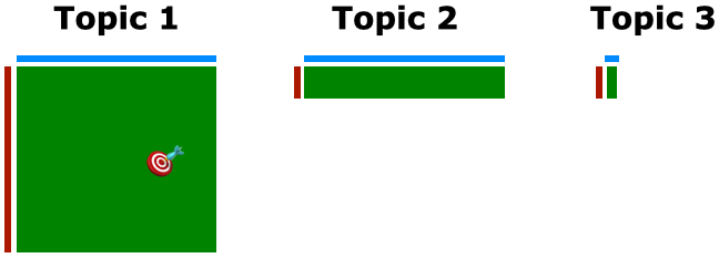
Human judgments: Word intrusion

Word intrusion: Take high probability words from a topic. Now add a high probability word from another topic to this topic.
Likely words from old topic
- dentist, appointment, doctors, tooth
Likely words from old topic + word intrusion
- dentist, mom, appointment, doctors, tooth
Are we able to distinguish this odd word out from the original topic?

Coherence model

Coherence models provide a framework to evaluate the coherence of the topic by measuring the degree of semantic similarity between most likely words in the topic.
You can calculate coherence scores using Gensim’s CoherenceModel.
- Ranges from -1 to 1
- Roughly, high coherence score means the topics are semantically interpretable and low coherence scores means they are not semantically similar.
Let’s try it out on our toy data.

# Compute Coherence Score
from gensim.models import CoherenceModel

K = [1, 2, 3, 4, 5, 6]

coherence_scores = []

for num_topics in K:
    lda = LdaModel(
        corpus=doc_term_matrix,
        id2word=dictionary,
        num_topics=num_topics,
        random_state=42,
        passes=10,
    )
    coherence_model_lda = CoherenceModel(
        model=lda, texts=corpus, dictionary=dictionary, coherence="c_v"
    )
    coherence_scores.append(coherence_model_lda.get_coherence())

df = pd.DataFrame(coherence_scores, index=K, columns=["Coherence score"])
df

	Coherence score
1	0.231307
2	0.273446
3	0.347582
4	0.611676
5	0.606312
6	0.492354

df.plot(title="Coherence scores", xlabel="num_topics", ylabel="Coherence score");

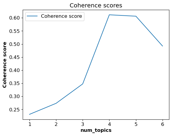
../../_images/58c2e5a135e47f4eac5900f04e225a1a6ccf5573a79fbe7fa34409dc3045de81.png

We are getting the best coherence score with num_topics = 4. That said, similar to other methods introduced as a guiding tool to choose the optimal hyperparameters, take this with a grain of salt. The model with highest coherence score is not necessarily going to be the best topic model. It’s always a good idea to manually examine the topics resulted by the chosen number of topics and examine whether you are able to make sense of these topics or or not before finalizing the number of topics. In the end our goal is to get human interpretable topics, and that’s what we should try to focus on.

If you want to jointly optimize num_topics, alpha, and eta, you can do grid search or random search with coherence score as the evaluation metric.

(Optional) Visualize topics

You can also visualize the topics using pyLDAvis.

pip install pyLDAvis

Do not install it using conda. They have made some changes in the recent version and conda build is not available for this version yet.

import warnings

warnings.filterwarnings("ignore", category=DeprecationWarning)

# import gensim
# import pyLDAvis.gensim_models as gensimvis
# import pyLDAvis

# vis = gensimvis.prepare(lda, doc_term_matrix, dictionary, sort_topics=False)
# pyLDAvis.display(vis)

4. (Optional) Some recent topic modeling tools#

4.1 Topic2Vec #

What are some limitations of LDA and LSA?

Need to know the number of topics in advance, which is hard for large and unfamiliar datasets
Quality of topics is very much dependent upon the quality of preprocessing
They use bag-of-words (BOW) representations of documents as input which ignore word semantics.
- The words study and studying would be treated as different words despite their semantic similarity
- Stemming or lemmatization can address this but lemmatization doesn’t help to recognize height and tall are similar

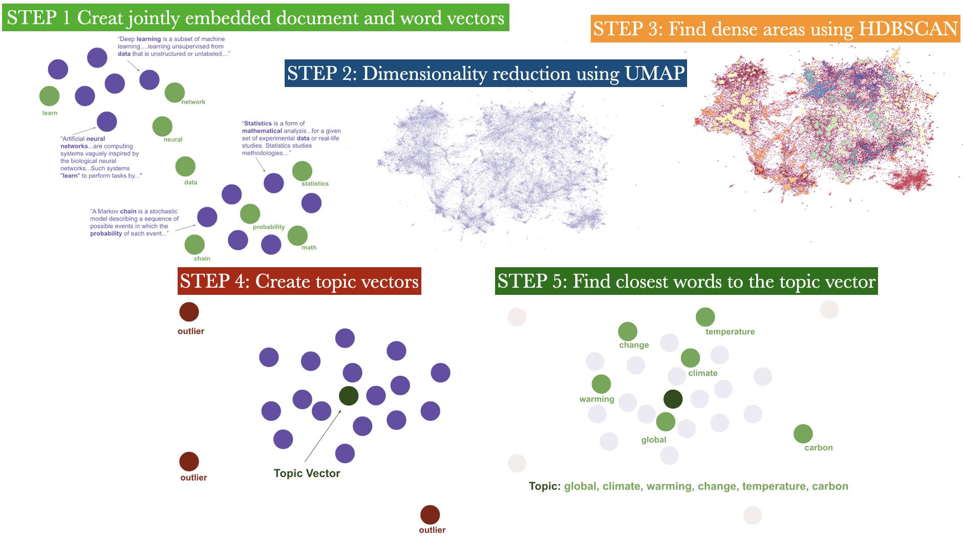
How does it work?

STEP 1: Create jointly embedded document and word vectors using Doc2Vec or Universal Sentence Encoder or BERT Sentence Transformer.
STEP 2: Create lower dimensional embedding of document vectors using UMAP.
STEP 3: Find dense areas of documents using HDBSCAN.
STEP 4: For each dense area calculate the centroid of document vectors in original dimension, this is the topic vector.
STEP 5: Find n-closest word vectors to the resulting topic vector.

Source

Let’s try it out to identify topics from Ted talk titles.

talks_df = pd.read_csv(DATA_DIR + '20221013_ted_talks.csv')
talks_df['title']

                        Averting the climate crisis
                                   Simplicity sells
                                Greening the ghetto
                    The best stats you've ever seen
                        Do schools kill creativity?
                             ...                      
                       Is inequality inevitable?
   4 ways to design a disability-friendly future
  Can exercise actually "boost" your metabolism?
   How did they build the Great Pyramid of Giza?
  How to squeeze all the juice out of retirement
Name: title, Length: 5701, dtype: object

documents = talks_df['title'].to_list()

from top2vec import Top2Vec

model = Top2Vec(documents,embedding_model='distiluse-base-multilingual-cased', min_count=5)

2025-03-05 08:39:10,456 - top2vec - INFO - Pre-processing documents for training
/Users/kvarada/miniforge3/envs/563/lib/python3.12/site-packages/sklearn/feature_extraction/text.py:517: UserWarning:

The parameter 'token_pattern' will not be used since 'tokenizer' is not None'

2025-03-05 08:39:10,517 - top2vec - INFO - Downloading distiluse-base-multilingual-cased model
2025-03-05 08:39:12,990 - top2vec - INFO - Creating joint document/word embedding
2025-03-05 08:39:20,352 - top2vec - INFO - Creating lower dimension embedding of documents
/Users/kvarada/miniforge3/envs/563/lib/python3.12/site-packages/sklearn/utils/deprecation.py:151: FutureWarning:

'force_all_finite' was renamed to 'ensure_all_finite' in 1.6 and will be removed in 1.8.

2025-03-05 08:39:29,490 - top2vec - INFO - Finding dense areas of documents
/Users/kvarada/miniforge3/envs/563/lib/python3.12/site-packages/sklearn/utils/deprecation.py:151: FutureWarning:

'force_all_finite' was renamed to 'ensure_all_finite' in 1.6 and will be removed in 1.8.

/Users/kvarada/miniforge3/envs/563/lib/python3.12/site-packages/sklearn/utils/deprecation.py:151: FutureWarning:

'force_all_finite' was renamed to 'ensure_all_finite' in 1.6 and will be removed in 1.8.

2025-03-05 08:39:29,618 - top2vec - INFO - Finding topics

# How many topics has it learned? 

model.get_num_topics() 

# What are the topic sizes? 

topic_sizes, topic_nums = model.get_topic_sizes()
topic_sizes

array([311, 283, 227, 197, 190, 144, 143, 138, 135, 134, 132, 131, 129,
       128, 126, 124, 122, 106, 105, 103,  97,  96,  94,  93,  92,  88,
        88,  86,  77,  76,  75,  74,  73,  70,  70,  68,  67,  66,  62,
        59,  59,  58,  57,  54,  54,  53,  53,  51,  51,  50,  49,  49,
        48,  46,  45,  45,  40,  36,  33,  33,  29,  29])

# What are the topic words? 

topic_words, word_scores, topic_nums = model.get_topics(1)
topic_words

array([['why', 'reasons', 'reason', 'causes', 'how', 'como', 'autism',
        'co', 'disease', 'diseases', 'what', 'anxiety', 'depression',
        'addiction', 'sick', 'habits', 'que', 'vaccines', 'fear',
        'hunger', 'hate', 'genetic', 'grief', 'cancer', 'vaccine',
        'pandemics', 'poverty', 'empathy', 'myths', 'about', 'weird',
        'when', 'for', 'pain', 'mysteries', 'crisis', 'alzheimer',
        'mental', 'drugs', 'brains', 'malaria', 'fallacy', 'who', 'tips',
        'never', 'hiv', 'strange', 'riddle', 'as', 'suicide']],
      dtype='<U14')

import warnings

warnings.filterwarnings("ignore", category=DeprecationWarning)

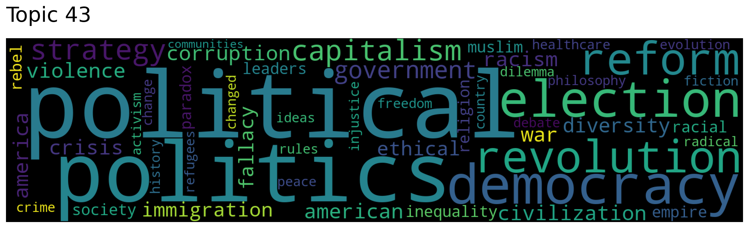
topic_words, word_scores, topic_scores, topic_nums = model.search_topics(keywords=["politics"], 
                                                                         num_topics=5)
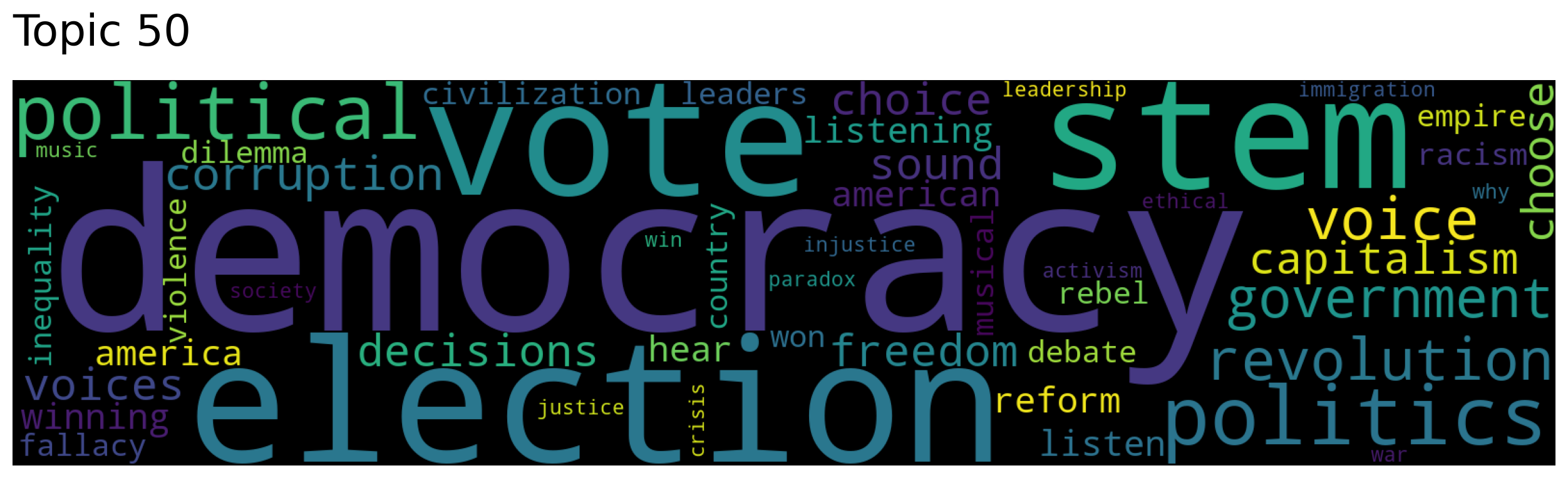
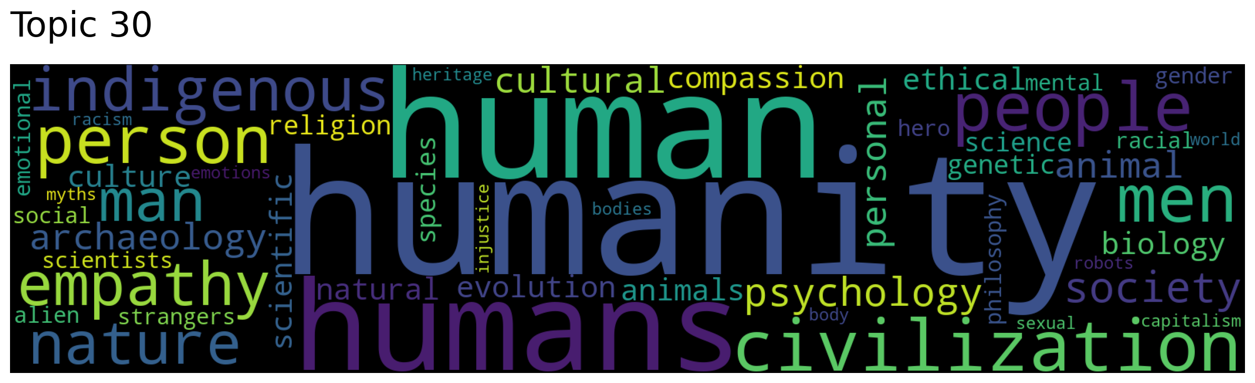
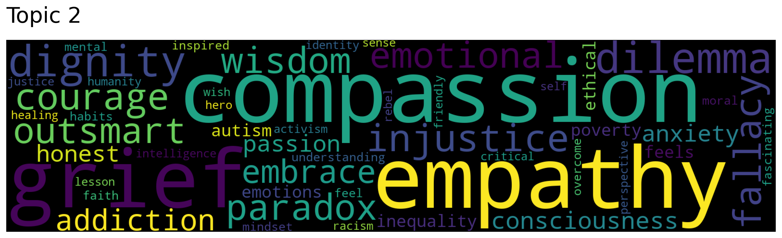
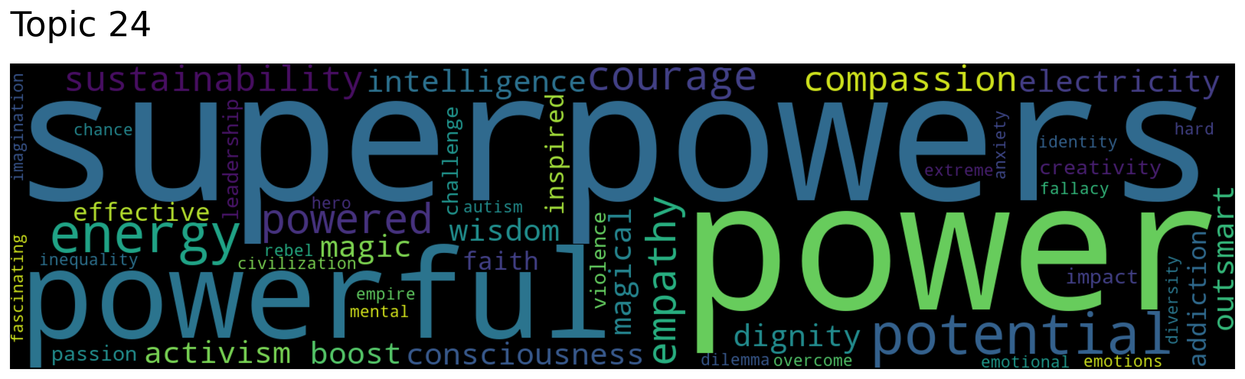
for topic in topic_nums:
    model.generate_topic_wordcloud(topic)

../../_images/ce5f30c0ee4ea03078ce3bbc8aa102e1a96182ed2a3c5b0bc7c6ee790c175d7f.png

../../_images/e517e207436b82b4b81d3944c96e5da3f916e9f465e45c5d8549998fdb27a5bd.png

../../_images/5e32100f6f90406843550442d5821cbecdea893a1d57809e06ff4c4437208096.png

../../_images/a3d9e5923334913b1ae5ac025f5b92283a915a802a8134d09c03a684aaa10945.png

../../_images/ae138ca0cf40be200438c89ec3deba1e309a633cad5c606ab4195b1f4aaad57e.png

documents, document_scores, document_ids = model.search_documents_by_topic(topic_num=26, num_docs=5)
for doc, score, doc_id in zip(documents, document_scores, document_ids):
    print(f"Document: {doc_id}, Score: {score}")
    print("-----------")
    print(doc)
    print("-----------")
    print()

Document: 4517, Score: 0.7487233877182007
-----------
The mental health benefits of storytelling for health care workers
-----------

Document: 5529, Score: 0.7033652663230896
-----------
Mental health care that disrupts cycles of violence
-----------

Document: 1319, Score: 0.6959103345870972
-----------
Mental health for all by involving all
-----------

Document: 2959, Score: 0.6899876594543457
-----------
How to do more with less in healthcare
-----------

Document: 3028, Score: 0.6870319247245789
-----------
Healthcare's compassion crisis
-----------

documents, document_scores, document_ids = model.search_documents_by_keywords(keywords=["human", "love"], num_docs=5)
for doc, score, doc_id in zip(documents, document_scores, document_ids):
    print(f"Document: {doc_id}, Score: {score}")
    print("-----------")
    print(doc)
    print("-----------")
    print()

Document: 264, Score: 0.67848694569802
-----------
On humanity
-----------

Document: 5309, Score: 0.5884557978425976
-----------
"Being Human"
-----------

Document: 258, Score: 0.5522820402610216
-----------
The brain in love
-----------

Document: 584, Score: 0.5464832461129183
-----------
The uniqueness of humans
-----------

Document: 4532, Score: 0.5446537307927031
-----------
The language of being human
-----------

topic_words, topic_vectors, topic_labels = model.get_topics()

topic_words

array([['why', 'reasons', 'reason', ..., 'riddle', 'as', 'suicide'],
       ['how', 'ways', 'como', ..., 'injustice', 'helps', 'work'],
       ['compassion', 'empathy', 'grief', ..., 'perspective', 'wish',
        'justice'],
       ...,
       ['leadership', 'leaders', 'guide', ..., 'boost', 'election',
        'path'],
       ['social', 'twitter', 'society', ..., 'ourselves', 'technology',
        'inventions'],
       ['why', 'read', 'reading', ..., 'tale', 'pandemics', 'quantum']],
      dtype='<U14')

Another recent tool to know is BERTopic, which leverages transformers.

Final comments and summary#

Important ideas to know#

Topic modeling is a tool to uncover important themes in a large collection of documents.
The overall goal is to tell a high-level story about a large collection of documents to humans.

(Credit: Health topics in social media)

Latent dirichlet allocation (LDA) is a commonly used model for topic modeling, which is a Bayesian, probabilistic, and generative model.
Topic is something that influences the choice of vocabulary of a document. For each document, we assume that several topics are active with varying importance.
The primary idea of the model is
- A document is a mixture of topics
- A topic is a mixture of words in the vocabulary

You can carry out topic modeling with LDA in Python using the Gensim library.
Preprocessing is extremely important in topic modeling.
Some of the most common steps in preprocessing for topic modeling include
- Sentence segmentation, tokenization, lemmatization, stopword and punctuation removal
You can visualize topic model using pyLDAvis.
There are more advanced and practical tools for topic modeling out there. Some examples include Top2Vec and BERTopic

Some useful resources and links#

LDA with sklearn
Jordan Boyd-Graber’s very approachable explanation of LDA
lda2vec
Original topic modeling paper: David Blei et al. 2003
Topic modeling for computational social scientists
spaCy’s Python for data science cheat sheet
If you want to learn more about practical aspects of LDA
- Rethinking LDA: Why Priors Matter
- LDA Revisited: Entropy, Prior and Convergence

Lecture 6: Topic Modeling

Contents

Lecture 6: Topic Modeling#

Imports, LO#

Imports#

Learning outcomes#

1. Why topic modeling?#

1.1 Topic modeling motivation#

1.2 How do you do topic modeling?#

2. Topic modeling with Latent Dirichlet Allocation (LDA)#

2.1 Possible approaches to generate documents#

2.2 Generative story of LDA#

2.3 LDA inference (high-level)#

❓❓ Questions for you#

Exercise: Select all of the following statements which are True (iClicker)#

Exercise: Questions for class discussion#

3. Topic modeling with Python#

3.1 Topic modeling pipeline#

3.2 A few comments on evaluation#

4. (Optional) Some recent topic modeling tools#

4.1 Topic2Vec#

Final comments and summary#

Important ideas to know#

Some useful resources and links#

4.1 Topic2Vec #