Appendix A: K-Means customer segmentation case study

import os
import random
import sys
import time

import numpy as np
import pandas as pd

import matplotlib.pyplot as plt
import seaborn as sns
sys.path.append(os.path.join(os.path.abspath(".."), "code"))
from plotting_functions import *

DATA_DIR = os.path.join(os.path.abspath(".."), "data/")
from sklearn import cluster, datasets, metrics
from sklearn.compose import ColumnTransformer, make_column_transformer
from sklearn.datasets import make_blobs
from sklearn.decomposition import PCA
from sklearn.pipeline import Pipeline, make_pipeline
from sklearn.preprocessing import StandardScaler
# from support_functions import *
from yellowbrick.cluster import KElbowVisualizer, SilhouetteVisualizer

#plt.style.use("seaborn")

plt.rcParams["font.size"] = 16

---------------------------------------------------------------------------
ImportError                               Traceback (most recent call last)
Cell In[1], line 12
     10 import seaborn as sns
     11 sys.path.append(os.path.join(os.path.abspath(".."), "code"))
---> 12 from plotting_functions import *
     14 DATA_DIR = os.path.join(os.path.abspath(".."), "data/")
     15 from sklearn import cluster, datasets, metrics

File ~/MDS/2024-25/563/DSCI_563_unsup-learn/lectures/code/plotting_functions.py:7
      5 import matplotlib.pyplot as plt
      6 from matplotlib.colors import ListedColormap, colorConverter, LinearSegmentedColormap
----> 7 from scipy.spatial import distance
      8 from sklearn.metrics import euclidean_distances
      9 from sklearn.manifold import MDS

File ~/miniforge3/envs/jbook/lib/python3.12/site-packages/scipy/spatial/__init__.py:110
      1 """
      2 =============================================================
      3 Spatial algorithms and data structures (:mod:`scipy.spatial`)
   (...)
    107    QhullError
    108 """  # noqa: E501
--> 110 from ._kdtree import *
    111 from ._ckdtree import *  # type: ignore[import-not-found]
    112 from ._qhull import *

File ~/miniforge3/envs/jbook/lib/python3.12/site-packages/scipy/spatial/_kdtree.py:4
      1 # Copyright Anne M. Archibald 2008
      2 # Released under the scipy license
      3 import numpy as np
----> 4 from ._ckdtree import cKDTree, cKDTreeNode  # type: ignore[import-not-found]
      6 __all__ = ['minkowski_distance_p', 'minkowski_distance',
      7            'distance_matrix',
      8            'Rectangle', 'KDTree']
     11 def minkowski_distance_p(x, y, p=2):

File _ckdtree.pyx:11, in init scipy.spatial._ckdtree()

File ~/miniforge3/envs/jbook/lib/python3.12/site-packages/scipy/sparse/__init__.py:315
    312 from ._sputils import get_index_dtype, safely_cast_index_arrays
    314 # For backward compatibility with v0.19.
--> 315 from . import csgraph
    317 # Deprecated namespaces, to be removed in v2.0.0
    318 from . import (
    319     base, bsr, compressed, construct, coo, csc, csr, data, dia, dok, extract,
    320     lil, sparsetools, sputils
    321 )

File ~/miniforge3/envs/jbook/lib/python3.12/site-packages/scipy/sparse/csgraph/__init__.py:187
    158 __docformat__ = "restructuredtext en"
    160 __all__ = ['connected_components',
    161            'laplacian',
    162            'shortest_path',
   (...)
    184            'csgraph_to_masked',
    185            'NegativeCycleError']
--> 187 from ._laplacian import laplacian
    188 from ._shortest_path import (
    189     shortest_path, floyd_warshall, dijkstra, bellman_ford, johnson, yen,
    190     NegativeCycleError
    191 )
    192 from ._traversal import (
    193     breadth_first_order, depth_first_order, breadth_first_tree,
    194     depth_first_tree, connected_components
    195 )

File ~/miniforge3/envs/jbook/lib/python3.12/site-packages/scipy/sparse/csgraph/_laplacian.py:7
      5 import numpy as np
      6 from scipy.sparse import issparse
----> 7 from scipy.sparse.linalg import LinearOperator
      8 from scipy.sparse._sputils import convert_pydata_sparse_to_scipy, is_pydata_spmatrix
     11 ###############################################################################
     12 # Graph laplacian

File ~/miniforge3/envs/jbook/lib/python3.12/site-packages/scipy/sparse/linalg/__init__.py:129
      1 """
      2 Sparse linear algebra (:mod:`scipy.sparse.linalg`)
      3 ==================================================
   (...)
    126 
    127 """
--> 129 from ._isolve import *
    130 from ._dsolve import *
    131 from ._interface import *

File ~/miniforge3/envs/jbook/lib/python3.12/site-packages/scipy/sparse/linalg/_isolve/__init__.py:4
      1 "Iterative Solvers for Sparse Linear Systems"
      3 #from info import __doc__
----> 4 from .iterative import *
      5 from .minres import minres
      6 from .lgmres import lgmres

File ~/miniforge3/envs/jbook/lib/python3.12/site-packages/scipy/sparse/linalg/_isolve/iterative.py:5
      3 from scipy.sparse.linalg._interface import LinearOperator
      4 from .utils import make_system
----> 5 from scipy.linalg import get_lapack_funcs
      7 __all__ = ['bicg', 'bicgstab', 'cg', 'cgs', 'gmres', 'qmr']
     10 def _get_atol_rtol(name, b_norm, atol=0., rtol=1e-5):

File ~/miniforge3/envs/jbook/lib/python3.12/site-packages/scipy/linalg/__init__.py:203
      1 """
      2 ====================================
      3 Linear algebra (:mod:`scipy.linalg`)
   (...)
    200 
    201 """  # noqa: E501
--> 203 from ._misc import *
    204 from ._cythonized_array_utils import *
    205 from ._basic import *

File ~/miniforge3/envs/jbook/lib/python3.12/site-packages/scipy/linalg/_misc.py:3
      1 import numpy as np
      2 from numpy.linalg import LinAlgError
----> 3 from .blas import get_blas_funcs
      4 from .lapack import get_lapack_funcs
      6 __all__ = ['LinAlgError', 'LinAlgWarning', 'norm']

File ~/miniforge3/envs/jbook/lib/python3.12/site-packages/scipy/linalg/blas.py:213
    210 import numpy as np
    211 import functools
--> 213 from scipy.linalg import _fblas
    214 try:
    215     from scipy.linalg import _cblas

ImportError: dlopen(/Users/kvarada/miniforge3/envs/jbook/lib/python3.12/site-packages/scipy/linalg/_fblas.cpython-312-darwin.so, 0x0002): Library not loaded: @rpath/libgfortran.5.dylib
  Referenced from: <0B9C315B-A1DD-3527-88DB-4B90531D343F> /Users/kvarada/miniforge3/envs/jbook/lib/libopenblas.0.dylib
  Reason: tried: '/Users/kvarada/miniforge3/envs/jbook/lib/libgfortran.5.dylib' (duplicate LC_RPATH '@loader_path'), '/Users/kvarada/miniforge3/envs/jbook/lib/libgfortran.5.dylib' (duplicate LC_RPATH '@loader_path'), '/Users/kvarada/miniforge3/envs/jbook/lib/python3.12/site-packages/scipy/linalg/../../../../libgfortran.5.dylib' (duplicate LC_RPATH '@loader_path'), '/Users/kvarada/miniforge3/envs/jbook/lib/python3.12/site-packages/scipy/linalg/../../../../libgfortran.5.dylib' (duplicate LC_RPATH '@loader_path'), '/Users/kvarada/miniforge3/envs/jbook/bin/../lib/libgfortran.5.dylib' (duplicate LC_RPATH '@loader_path'), '/Users/kvarada/miniforge3/envs/jbook/bin/../lib/libgfortran.5.dylib' (duplicate LC_RPATH '@loader_path'), '/usr/local/lib/libgfortran.5.dylib' (no such file), '/usr/lib/libgfortran.5.dylib' (no such file, not in dyld cache)

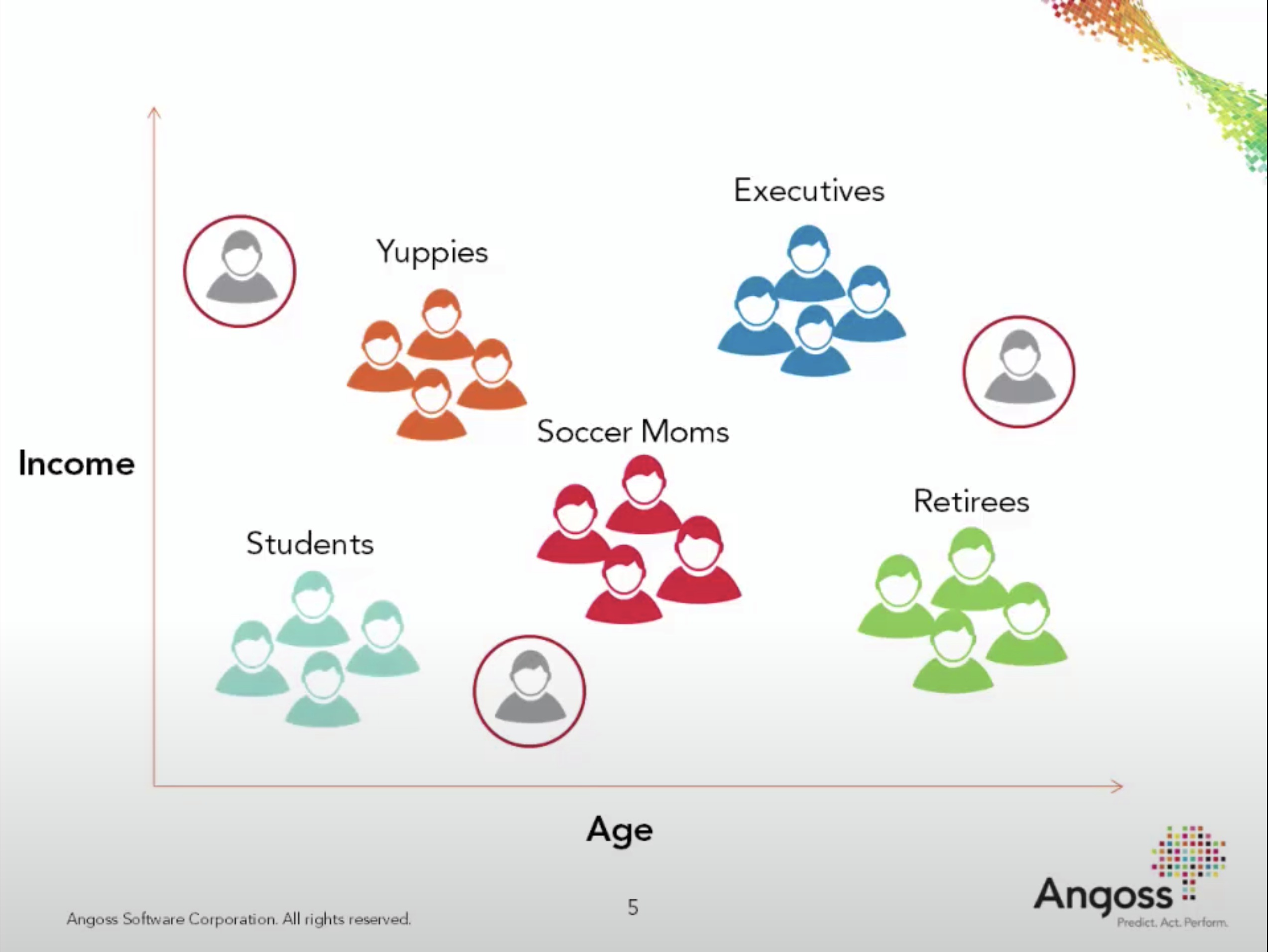
What is customer segmentation?

• Understand landscape of the market in businesses and craft targeted business or marketing strategies tailored for each group.

source

Check out this interesting talk by Malcom Gladwell. Humans are diverse and there is no single spaghetti sauce that would make all of them happy!

Often it’s beneficial to businesses to explore the landscape of the market and tailor their services and products offered to each group. This is called customer segmentation. It’s usually applied when the dataset contains some of the following features.

• Demographic information such as gender, age, marital status, income, education, and occupation

• Geographical information such as specific towns or counties or a customer’s city, state, or even country of residence (in case of big global companies)

• Psychographics such as social class, lifestyle, and personality traits

• Behavioral data such as spending and consumption habits, product/service usage, and desired benefits

Business problem

• Imagine that you are hired as a data scientist at a bank. They provide some data of their credit card customers to you.

• Their goal is to develop customized marketing campaigns and they ask you to group customers based on the given information.

• Now that you know about K-Means clustering, let’s apply it to the dataset to group customers.

Data

• We will use the Credit Card Dataset for clustering from Kaggle.

• Download the data and save the CSV under the data folder.

• I encourage you to work through this case study on your own.

creditcard_df = pd.read_csv(DATA_DIR + "CC General.csv")
creditcard_df.shape

(8950, 18)

Information of the dataset

We have behavioral data.

• CUSTID: Identification of Credit Card holder

• BALANCE: Balance amount left in customer’s account to make purchases

• BALANCE_FREQUENCY: How frequently the Balance is updated, score between 0 and 1 (1 = frequently updated, 0 = not frequently updated)

• PURCHASES: Amount of purchases made from account

• ONEOFFPURCHASES: Maximum purchase amount done in one-go

• INSTALLMENTS_PURCHASES: Amount of purchase done in installment

• CASH_ADVANCE: Cash in advance given by the user

• PURCHASES_FREQUENCY: How frequently the Purchases are being made, score between 0 and 1 (1 = frequently purchased, 0 = not frequently purchased)

• ONEOFF_PURCHASES_FREQUENCY: How frequently Purchases are happening in one-go (1 = frequently purchased, 0 = not frequently purchased)

• PURCHASES_INSTALLMENTS_FREQUENCY: How frequently purchases in installments are being done (1 = frequently done, 0 = not frequently done)

• CASH_ADVANCE_FREQUENCY: How frequently the cash in advance being paid

• CASH_ADVANCE_TRX: Number of Transactions made with “Cash in Advance”

• PURCHASES_TRX: Number of purchase transactions made

• CREDIT_LIMIT: Limit of Credit Card for user

• PAYMENTS: Amount of Payment done by user

• MINIMUM_PAYMENTS: Minimum amount of payments made by user

• PRC_FULL_PAYMENT: Percent of full payment paid by user

• TENURE: Tenure of credit card service for user

Preliminary EDA

creditcard_df.info()

<class 'pandas.core.frame.DataFrame'>
RangeIndex: 8950 entries, 0 to 8949
Data columns (total 18 columns):
 #   Column                            Non-Null Count  Dtype  
---  ------                            --------------  -----  
 0   CUST_ID                           8950 non-null   object 
 1   BALANCE                           8950 non-null   float64
 2   BALANCE_FREQUENCY                 8950 non-null   float64
 3   PURCHASES                         8950 non-null   float64
 4   ONEOFF_PURCHASES                  8950 non-null   float64
 5   INSTALLMENTS_PURCHASES            8950 non-null   float64
 6   CASH_ADVANCE                      8950 non-null   float64
 7   PURCHASES_FREQUENCY               8950 non-null   float64
 8   ONEOFF_PURCHASES_FREQUENCY        8950 non-null   float64
 9   PURCHASES_INSTALLMENTS_FREQUENCY  8950 non-null   float64
 10  CASH_ADVANCE_FREQUENCY            8950 non-null   float64
 11  CASH_ADVANCE_TRX                  8950 non-null   int64  
 12  PURCHASES_TRX                     8950 non-null   int64  
 13  CREDIT_LIMIT                      8949 non-null   float64
 14  PAYMENTS                          8950 non-null   float64
 15  MINIMUM_PAYMENTS                  8637 non-null   float64
 16  PRC_FULL_PAYMENT                  8950 non-null   float64
 17  TENURE                            8950 non-null   int64  
dtypes: float64(14), int64(3), object(1)
memory usage: 1.2+ MB

• All numeric features

• Some missing values

creditcard_df.describe()

	BALANCE	BALANCE_FREQUENCY	PURCHASES	ONEOFF_PURCHASES	INSTALLMENTS_PURCHASES	CASH_ADVANCE	PURCHASES_FREQUENCY	ONEOFF_PURCHASES_FREQUENCY	PURCHASES_INSTALLMENTS_FREQUENCY	CASH_ADVANCE_FREQUENCY	CASH_ADVANCE_TRX	PURCHASES_TRX	CREDIT_LIMIT	PAYMENTS	MINIMUM_PAYMENTS	PRC_FULL_PAYMENT	TENURE
count	8950.000000	8950.000000	8950.000000	8950.000000	8950.000000	8950.000000	8950.000000	8950.000000	8950.000000	8950.000000	8950.000000	8950.000000	8949.000000	8950.000000	8637.000000	8950.000000	8950.000000
mean	1564.474828	0.877271	1003.204834	592.437371	411.067645	978.871112	0.490351	0.202458	0.364437	0.135144	3.248827	14.709832	4494.449450	1733.143852	864.206542	0.153715	11.517318
std	2081.531879	0.236904	2136.634782	1659.887917	904.338115	2097.163877	0.401371	0.298336	0.397448	0.200121	6.824647	24.857649	3638.815725	2895.063757	2372.446607	0.292499	1.338331
min	0.000000	0.000000	0.000000	0.000000	0.000000	0.000000	0.000000	0.000000	0.000000	0.000000	0.000000	0.000000	50.000000	0.000000	0.019163	0.000000	6.000000
25%	128.281915	0.888889	39.635000	0.000000	0.000000	0.000000	0.083333	0.000000	0.000000	0.000000	0.000000	1.000000	1600.000000	383.276166	169.123707	0.000000	12.000000
50%	873.385231	1.000000	361.280000	38.000000	89.000000	0.000000	0.500000	0.083333	0.166667	0.000000	0.000000	7.000000	3000.000000	856.901546	312.343947	0.000000	12.000000
75%	2054.140036	1.000000	1110.130000	577.405000	468.637500	1113.821139	0.916667	0.300000	0.750000	0.222222	4.000000	17.000000	6500.000000	1901.134317	825.485459	0.142857	12.000000
max	19043.138560	1.000000	49039.570000	40761.250000	22500.000000	47137.211760	1.000000	1.000000	1.000000	1.500000	123.000000	358.000000	30000.000000	50721.483360	76406.207520	1.000000	12.000000

Practice exercises for you

1. What is the average BALANCE amount?

2. How often the BALANCE_FREQUENCY is updated on average?

3. Obtain the row the customer who made the maximum cash advance transaction.

Mini exercises for you (Answers)

1. What is the average BALANCE amount? 1564.47

2. How often the BALANCE_FREQUENCY is updated on average? 0.877 (pretty often)

3. Obtain the row of the customer who made the maximum cash advance transaction.

# Answer 3.
max_cash_advance = creditcard_df["CASH_ADVANCE"].max()
creditcard_df[creditcard_df["CASH_ADVANCE"] == max_cash_advance]

	CUST_ID	BALANCE	BALANCE_FREQUENCY	PURCHASES	ONEOFF_PURCHASES	INSTALLMENTS_PURCHASES	CASH_ADVANCE	PURCHASES_FREQUENCY	ONEOFF_PURCHASES_FREQUENCY	PURCHASES_INSTALLMENTS_FREQUENCY	CASH_ADVANCE_FREQUENCY	CASH_ADVANCE_TRX	PURCHASES_TRX	CREDIT_LIMIT	PAYMENTS	MINIMUM_PAYMENTS	PRC_FULL_PAYMENT	TENURE
2159	C12226	10905.05381	1.0	431.93	133.5	298.43	47137.21176	0.583333	0.25	0.5	1.0	123	21	19600.0	39048.59762	5394.173671	0.0	12

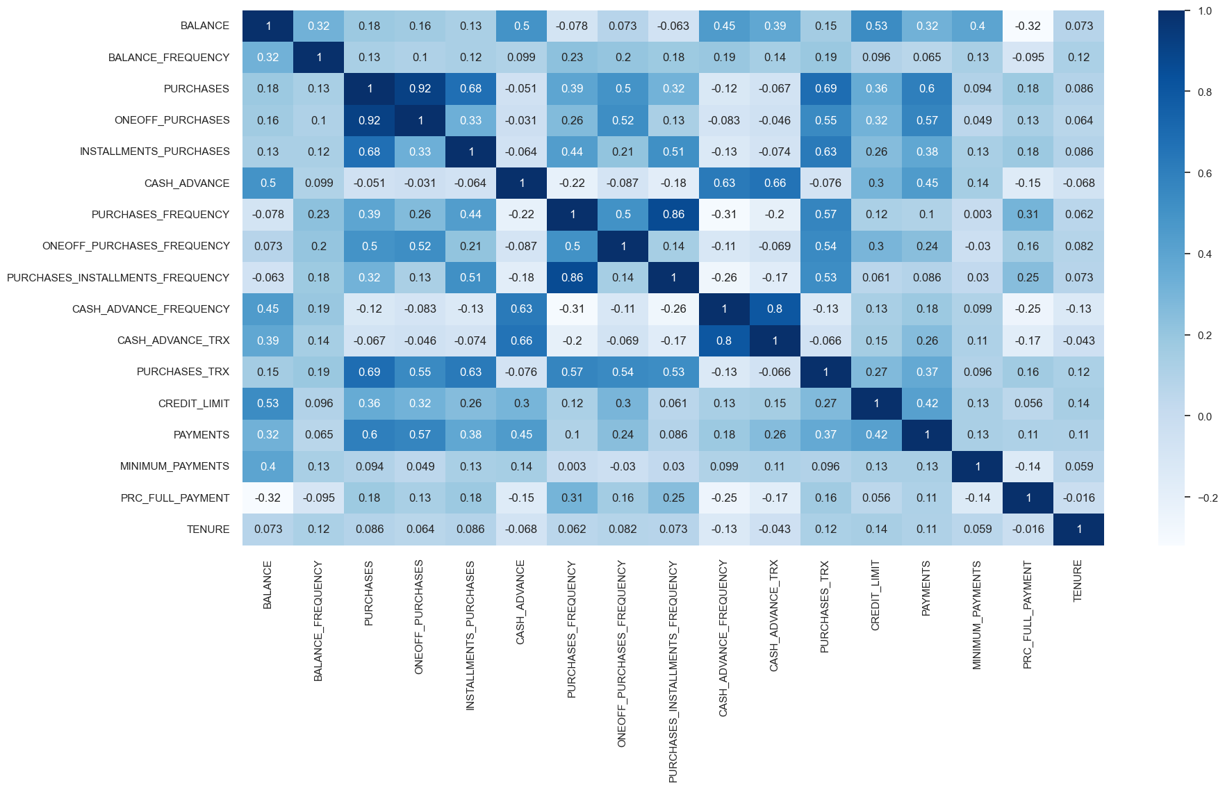
Let’s examine correlations between features.

cor = creditcard_df.corr(numeric_only=True)
plt.figure(figsize=(20, 10))
sns.set(font_scale=1)
sns.heatmap(cor, annot=True, cmap=plt.cm.Blues);

Feature types and preprocessing

Let’s identify different feature types and transformations

creditcard_df.columns

Index(['CUST_ID', 'BALANCE', 'BALANCE_FREQUENCY', 'PURCHASES',
       'ONEOFF_PURCHASES', 'INSTALLMENTS_PURCHASES', 'CASH_ADVANCE',
       'PURCHASES_FREQUENCY', 'ONEOFF_PURCHASES_FREQUENCY',
       'PURCHASES_INSTALLMENTS_FREQUENCY', 'CASH_ADVANCE_FREQUENCY',
       'CASH_ADVANCE_TRX', 'PURCHASES_TRX', 'CREDIT_LIMIT', 'PAYMENTS',
       'MINIMUM_PAYMENTS', 'PRC_FULL_PAYMENT', 'TENURE'],
      dtype='object')

drop_features = ["CUST_ID"]
numeric_features = list(set(creditcard_df.columns) - set(drop_features))

from sklearn.impute import SimpleImputer

numeric_transformer = make_pipeline(SimpleImputer(), StandardScaler())

preprocessor = make_column_transformer(
    (numeric_transformer, numeric_features), ("drop", drop_features)
)

transformed_df = pd.DataFrame(
    data=preprocessor.fit_transform(creditcard_df), columns=numeric_features
)

transformed_df

	PURCHASES_TRX	INSTALLMENTS_PURCHASES	CASH_ADVANCE	PURCHASES	TENURE	CREDIT_LIMIT	CASH_ADVANCE_TRX	PURCHASES_INSTALLMENTS_FREQUENCY	PAYMENTS	MINIMUM_PAYMENTS	ONEOFF_PURCHASES	ONEOFF_PURCHASES_FREQUENCY	BALANCE_FREQUENCY	CASH_ADVANCE_FREQUENCY	BALANCE	PRC_FULL_PAYMENT	PURCHASES_FREQUENCY
0	-0.511333	-0.349079	-0.466786	-0.424900	0.360680	-0.960433	-0.476070	-0.707313	-0.528979	-3.109675e-01	-0.356934	-0.678661	-0.249434	-0.675349	-0.731989	-0.525551	-0.806490
1	-0.591796	-0.454576	2.605605	-0.469552	0.360680	0.688639	0.110074	-0.916995	0.818642	8.931021e-02	-0.356934	-0.678661	0.134325	0.573963	0.786961	0.234227	-1.221758
2	-0.109020	-0.454576	-0.466786	-0.107668	0.360680	0.826062	-0.476070	-0.916995	-0.383805	-1.016632e-01	0.108889	2.673451	0.518084	-0.675349	0.447135	-0.525551	1.269843
3	-0.551565	-0.454576	-0.368653	0.232058	0.360680	0.826062	-0.329534	-0.916995	-0.598688	4.878305e-17	0.546189	-0.399319	-1.016953	-0.258913	0.049099	-0.525551	-1.014125
4	-0.551565	-0.454576	-0.466786	-0.462063	0.360680	-0.905464	-0.476070	-0.916995	-0.364368	-2.657913e-01	-0.347294	-0.399319	0.518084	-0.675349	-0.358775	-0.525551	-1.014125
...	...	...	...	...	...	...	...	...	...	...	...	...	...	...	...	...	...
8945	-0.350408	-0.132643	-0.466786	-0.333293	-4.122768	-0.960433	-0.476070	1.179833	-0.486217	-3.498541e-01	-0.356934	-0.678661	0.518084	-0.675349	-0.737950	1.183951	1.269843
8946	-0.350408	-0.122823	-0.466786	-0.329136	-4.122768	-0.960433	-0.476070	1.179833	-0.503396	4.878305e-17	-0.356934	-0.678661	0.518084	-0.675349	-0.742423	-0.525551	1.269843
8947	-0.390639	-0.294893	-0.466786	-0.401965	-4.122768	-0.960433	-0.476070	0.760469	-0.570615	-3.354655e-01	-0.356934	-0.678661	-0.185477	-0.675349	-0.740398	0.329200	0.854576
8948	-0.591796	-0.454576	-0.449352	-0.469552	-4.122768	-1.097856	-0.182998	-0.916995	-0.580536	-3.469065e-01	-0.356934	-0.678661	-0.185477	0.157527	-0.745174	0.329200	-1.221758
8949	0.333524	-0.454576	-0.406205	0.042146	-4.122768	-0.905464	-0.182998	-0.916995	-0.576869	-3.329464e-01	0.301732	1.556082	-0.889033	0.990398	-0.572575	-0.525551	0.439310

8950 rows × 17 columns

Now that we have transformed the data, we are ready to run K-Means to cluster credit card customers.

Choosing n_clusters

• There is no definitive method to find the optimal number of clusters.

• Let’s try different approaches.

The Elbow method

model = KMeans(random_state=42, n_init='auto')
visualizer = KElbowVisualizer(model, k=(1, 20))

visualizer.fit(transformed_df)  # Fit the data to the visualizer
visualizer.show();

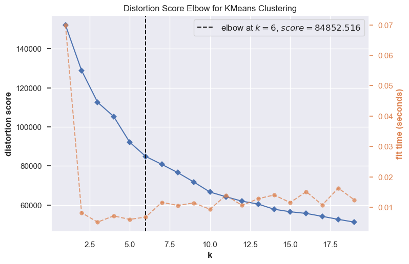
• The optimal number of clusters is not as clear as it was in our toy example.

• Let’s examine Silhouette scores.

for k in range(3, 6):
    model = KMeans(k, random_state=42)
    visualizer = SilhouetteVisualizer(model, colors="yellowbrick")
    visualizer.fit(transformed_df)  # Fit the data to the visualizer
    visualizer.show()

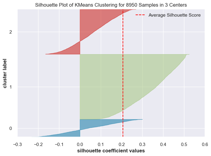
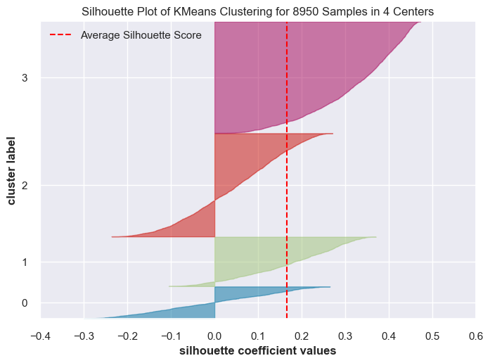
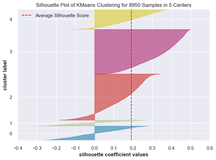
• I’m going to run KMeans with n_clusters = 4.

• You can try out n_clusters = 5 and n_clusters = 6 on your own.

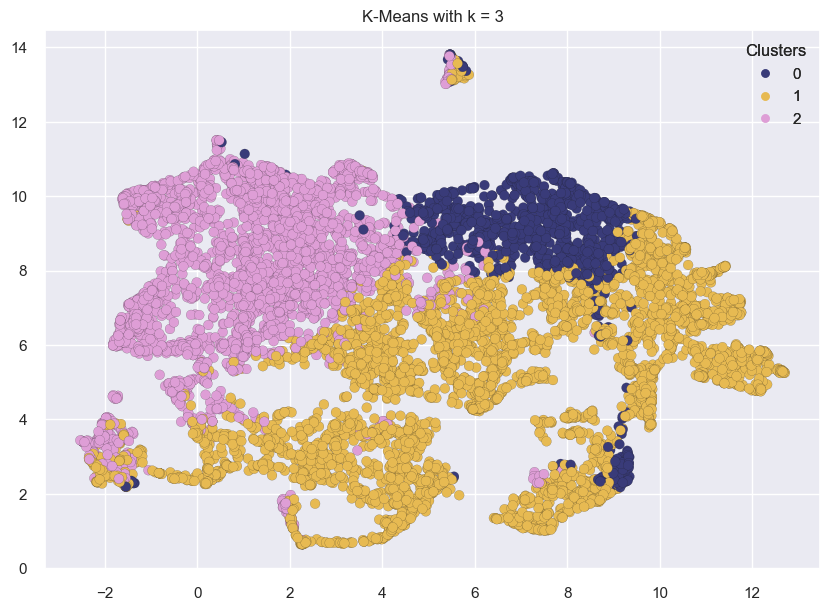
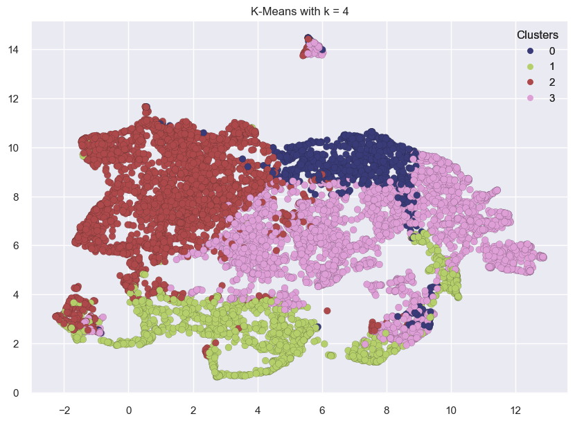
Visualizing clusters

• Can we visualize the clusters?

• We have a high dimensional data and we need to reduce the dimensionality in order to visualize it.

• Let’s reduce the dimensionality using a technique called UMAP.

I forgot to put this package in the course environment file. So to run the code below, you’ll have to install the umap-learn package in the course conda environment either with conda or pip, as described in the documentation.

> conda activate 563
> conda install -c conda-forge umap-learn

or

> conda activate 563
> pip install umap-learn

import umap

def plot_umap_clusters(
    data,
    cluster_labels,
    size=50,
    n_neighbors=15,
    title="UMAP visualization",
):
    """
    Carry out dimensionality reduction using UMAP and plot 2-dimensional clusters.

    Parameters
    -----------
    data : numpy array
        data as a numpy array
    cluster_labels : list
        cluster labels for each row in the dataset
    size : int
        size of points in the scatterplot
    n_neighbors : int
        n_neighbors hyperparameter of UMAP. See the documentation.
    title : str
        title for the visualization plot

    Returns
    -----------
    None. Shows the clusters.
    """

    reducer = umap.UMAP(n_neighbors=n_neighbors)
    Z = reducer.fit_transform(data)  # reduce dimensionality
    umap_df = pd.DataFrame(data=Z, columns=["dim1", "dim2"])
    umap_df["cluster"] = cluster_labels

    labels = np.unique(umap_df["cluster"])

    fig, ax = plt.subplots(figsize=(10, 7))
    ax.set_title(title)

    scatter = ax.scatter(
        umap_df["dim1"],
        umap_df["dim2"],
        c=umap_df["cluster"],
        cmap="tab20b",
        s=size,
        edgecolors="k",
        linewidths=0.1,
    )

    legend = ax.legend(*scatter.legend_elements(), loc="best", title="Clusters")
    ax.add_artist(legend)

    plt.show()

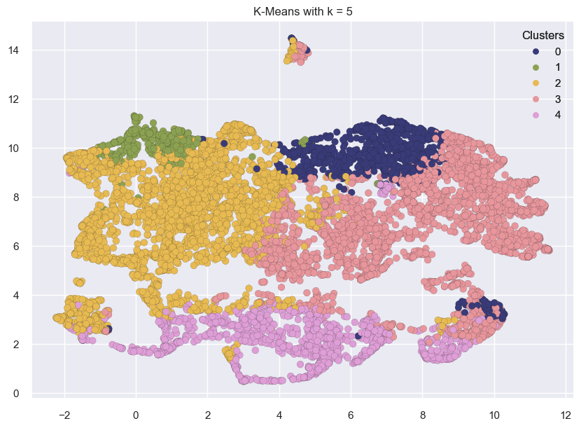
for k in range(3, 7):
    kmeans = KMeans(n_clusters=k, random_state=42)
    kmeans.fit(transformed_df)
    labels = kmeans.labels_
    plot_umap_clusters(transformed_df, kmeans.labels_, title=f"K-Means with k = {k}")

/Users/kvarada/miniforge3/envs/563/lib/python3.12/site-packages/sklearn/utils/deprecation.py:151: FutureWarning:

'force_all_finite' was renamed to 'ensure_all_finite' in 1.6 and will be removed in 1.8.

/Users/kvarada/miniforge3/envs/563/lib/python3.12/site-packages/sklearn/utils/deprecation.py:151: FutureWarning:

'force_all_finite' was renamed to 'ensure_all_finite' in 1.6 and will be removed in 1.8.

/Users/kvarada/miniforge3/envs/563/lib/python3.12/site-packages/sklearn/utils/deprecation.py:151: FutureWarning:

'force_all_finite' was renamed to 'ensure_all_finite' in 1.6 and will be removed in 1.8.

/Users/kvarada/miniforge3/envs/563/lib/python3.12/site-packages/sklearn/utils/deprecation.py:151: FutureWarning:

'force_all_finite' was renamed to 'ensure_all_finite' in 1.6 and will be removed in 1.8.

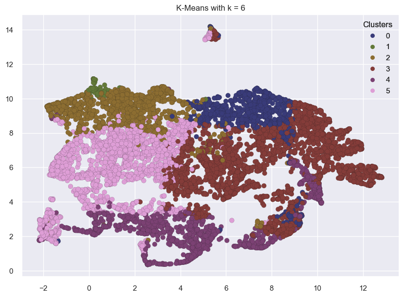
• The clusters above look reasonably well separated.

• This might not always be the case.

Cluster interpretation

• Let’s examine the cluster centers for k=4 and identify types of customers.

reasonable_k = 4
kmeans = KMeans(n_clusters=reasonable_k, random_state=42)
kmeans.fit(transformed_df)
labels = kmeans.labels_

cluster_centers = pd.DataFrame(
    data=kmeans.cluster_centers_, columns=[transformed_df.columns]
)
cluster_centers

	PURCHASES_TRX	INSTALLMENTS_PURCHASES	CASH_ADVANCE	PURCHASES	TENURE	CREDIT_LIMIT	CASH_ADVANCE_TRX	PURCHASES_INSTALLMENTS_FREQUENCY	PAYMENTS	MINIMUM_PAYMENTS	ONEOFF_PURCHASES	ONEOFF_PURCHASES_FREQUENCY	BALANCE_FREQUENCY	CASH_ADVANCE_FREQUENCY	BALANCE	PRC_FULL_PAYMENT	PURCHASES_FREQUENCY
0	-0.171033	-0.157231	1.955351	-0.130672	-0.077145	1.028456	1.846509	-0.360719	0.844275	0.587979	-0.082658	-0.135258	0.379847	1.876058	1.668482	-0.388985	-0.398442
1	-0.398135	-0.276859	-0.323962	-0.304986	-0.227297	-0.238330	-0.368721	-0.324939	-0.240955	-0.262345	-0.241643	-0.434756	-1.959157	-0.499183	-0.699072	0.339213	-0.421838
2	0.724525	0.585261	-0.354967	0.551465	0.157039	0.172113	-0.357770	0.965455	0.143300	-0.034300	0.390972	0.628970	0.411562	-0.466944	-0.149443	0.441615	1.091535
3	-0.444873	-0.373694	-0.088460	-0.337608	-0.022578	-0.348272	-0.034898	-0.645713	-0.267719	-0.020631	-0.230970	-0.350561	0.377251	0.115300	-0.030426	-0.447004	-0.708633

• Recall that we have applied imputation and scaling on the dataset.

• But we would be able to interpret these clusters better if the centers are in the original scale.

• So let’s apply inverse transformations to get the cluster center values in the original scale.

data = (
    preprocessor.named_transformers_["pipeline"]
    .named_steps["standardscaler"]
    .inverse_transform(cluster_centers[numeric_features])
)

org_cluster_centers = pd.DataFrame(data=data, columns=numeric_features)
org_cluster_centers = org_cluster_centers.reindex(
    sorted(org_cluster_centers.columns), axis=1
)
org_cluster_centers

	BALANCE	BALANCE_FREQUENCY	CASH_ADVANCE	CASH_ADVANCE_FREQUENCY	CASH_ADVANCE_TRX	CREDIT_LIMIT	INSTALLMENTS_PURCHASES	MINIMUM_PAYMENTS	ONEOFF_PURCHASES	ONEOFF_PURCHASES_FREQUENCY	PAYMENTS	PRC_FULL_PAYMENT	PURCHASES	PURCHASES_FREQUENCY	PURCHASES_INSTALLMENTS_FREQUENCY	PURCHASES_TRX	TENURE
0	5037.279872	0.967253	5079.333901	0.510563	15.849896	8236.391869	268.885549	2234.467700	455.241325	0.162108	4177.236119	0.039943	724.021625	0.330436	0.221079	10.458592	11.414079
1	109.416344	0.413164	299.507902	0.035253	0.732574	3627.308985	160.707741	252.821490	191.358908	0.072762	1035.603761	0.252929	351.597815	0.321047	0.235298	4.813673	11.213137
2	1253.422099	0.974766	234.489319	0.041704	0.807310	5120.665715	940.311888	784.272825	1241.370362	0.390092	2147.982881	0.282880	2181.418772	0.928436	0.748134	32.718820	11.727477
3	1501.145757	0.966638	793.365530	0.158217	3.010673	3227.295187	73.140602	816.126935	209.074918	0.097879	958.122729	0.022974	281.900172	0.205942	0.107815	3.651942	11.487103

cluster_labels = {0: "Transactors", 1: "Revolvers", 2: "Low activity", 3: "VIP/Prime"}
org_cluster_centers["cluster_labels"] = list(cluster_labels.values())

relevant_cols = [
    "cluster_labels",
    "BALANCE",
    "CREDIT_LIMIT",
    "PRC_FULL_PAYMENT",
    "PURCHASES_FREQUENCY",
    "CASH_ADVANCE",
    "CASH_ADVANCE_FREQUENCY",
    "CASH_ADVANCE_TRX",
]
org_cluster_centers[relevant_cols]

	cluster_labels	BALANCE	CREDIT_LIMIT	PRC_FULL_PAYMENT	PURCHASES_FREQUENCY	CASH_ADVANCE	CASH_ADVANCE_FREQUENCY	CASH_ADVANCE_TRX
0	Transactors	5037.279872	8236.391869	0.039943	0.330436	5079.333901	0.510563	15.849896
1	Revolvers	109.416344	3627.308985	0.252929	0.321047	299.507902	0.035253	0.732574
2	Low activity	1253.422099	5120.665715	0.282880	0.928436	234.489319	0.041704	0.807310
3	VIP/Prime	1501.145757	3227.295187	0.022974	0.205942	793.365530	0.158217	3.010673

One way to interpret and label the clusters above is as follows.

Transactors

• Credit card users who pay off their balance every month with least amount of interest charges.

• They are careful with their money.

• They have lowest balance and cash advance

Revolvers

• Credit card users who pay off only part of their monthly balance. They use credit card as a loan.

• They have highest balance and cash advance, high cash advance frequency, low purchase frequency, high cash advance transactions, low percentage of full payment

• Their credit limit is also high. (Lucrative group for banks 😟.)

Low activity

• There is not much activity in the account. It has low balance and not many purchases.

• Credit card users who have low credit limit.

VIP/Prime

• Credit card users who have high credit limit.

• They have high one-off purchases frequency, high number of purchase transactions.

• They have high balance but they also have higher percentage of full payment, similar to transactors

• Target for increase credit limit (and increase spending habits)

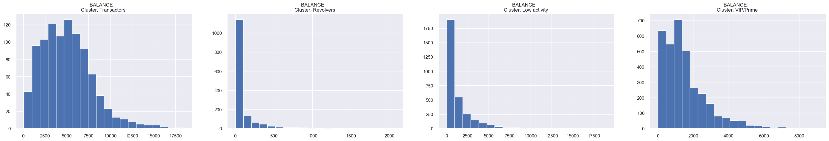
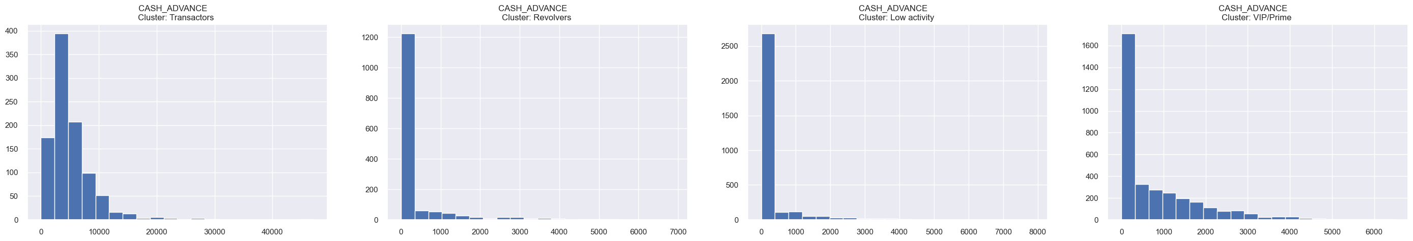
More on interpretation of clusters

• In real life, you’ll look through all features in detail before assigning meaning to clusters.

• This is not that easy, especially when you have a large number of features and clusters.

• One way to approach this would be visualizing the distribution of feature values for each cluster.

• Some domain knowledge would definitely help at this stage.

creditcard_df['cluster'] = labels

Let’s check the cluster assignment for the customer who made the maximum cash advance transaction.

creditcard_df[creditcard_df["CASH_ADVANCE"] == max_cash_advance] 

	CUST_ID	BALANCE	BALANCE_FREQUENCY	PURCHASES	ONEOFF_PURCHASES	INSTALLMENTS_PURCHASES	CASH_ADVANCE	PURCHASES_FREQUENCY	ONEOFF_PURCHASES_FREQUENCY	PURCHASES_INSTALLMENTS_FREQUENCY	CASH_ADVANCE_FREQUENCY	CASH_ADVANCE_TRX	PURCHASES_TRX	CREDIT_LIMIT	PAYMENTS	MINIMUM_PAYMENTS	PRC_FULL_PAYMENT	TENURE	cluster
2159	C12226	10905.05381	1.0	431.93	133.5	298.43	47137.21176	0.583333	0.25	0.5	1.0	123	21	19600.0	39048.59762	5394.173671	0.0	12	0

def show_hists(df=creditcard_df, cols=["BALANCE", "CASH_ADVANCE"]):
    for i in cols:
        plt.figure(figsize=(35, 5))
        for j in range(4):
            plt.subplot(1, 4, j + 1)
            cluster = df[df["cluster"] == j]
            cluster[i].hist(bins=20)
            plt.title(f"{i}    \nCluster: {cluster_labels[j]} ")

        plt.show()

show_hists() # Examining clusters for two features. 

# Uncomment the code below to show histograms for all features. 
# cols = creditcard_df_cluster.columns.to_list()
# cols.remove('CUST_ID')
# cols.remove('cluster')
# show_hists(creditcard_df_cluster, cols)

Practice exercise for you

• Try out different values for n_clusters in KMeans and examine the clusters.

• If you are feeling adventurous, you may try customer segmentation on All Lending Club loan data.