Connectivity Visualizations
Connectivity plots
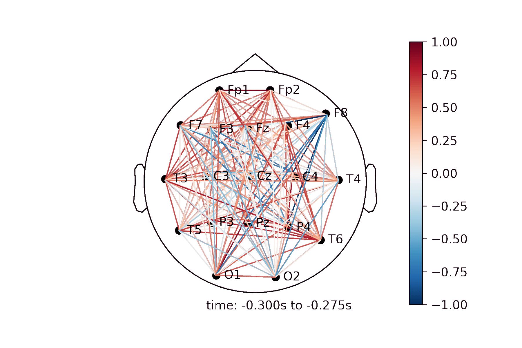
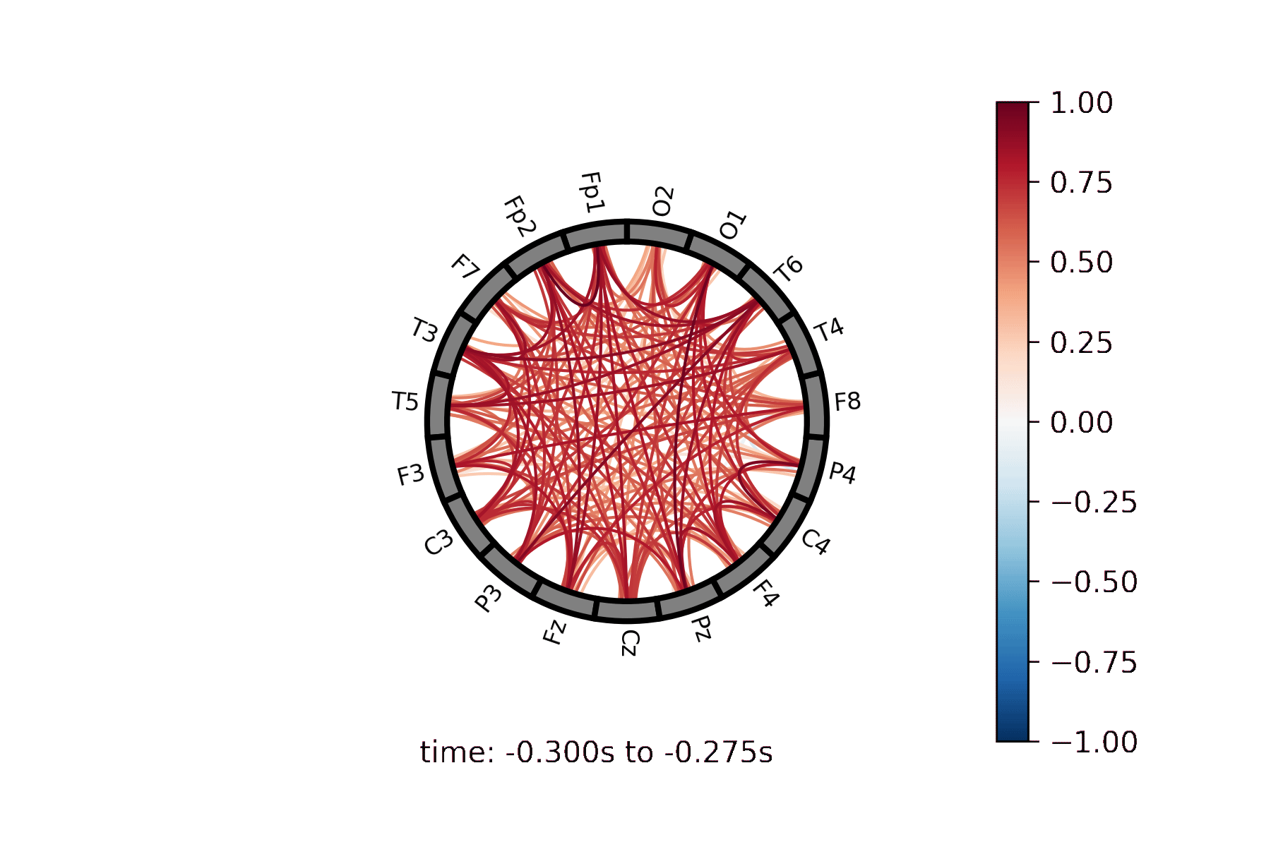
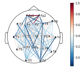
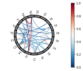
The connectivity plots provide a way to visualize pair-wise correlation, coherence, and connectivity measures between nodes. There are 2 types of plots, shown in the image below. Both types of plots can be generated as an animation to view changes over time or as standalone plots.
Lines drawn on a 2D representation of a skull |
Lines drawn between nodes represented in a circle |
General Setup
Import required modules
from simpl_eeg import connectivity, eeg_objects
import warnings
warnings.filterwarnings('ignore')
Create epoched data
For additional options see Creating EEG Objects section.
experiment_folder = "../../data/927"
nth_epoch = 0

epochs = eeg_objects.Epochs(experiment_folder)
epoch = epochs.get_epoch(nth_epoch)
Reading /Users/mpin/Documents/MDS/capstone/simpl_eeg_capstone/data/927/fixica.fdt
loaded raw from ../../data/927/fixica.set
Not setting metadata
Not setting metadata
33 matching events found
Setting baseline interval to [-0.2998046875, 0.0] sec
Applying baseline correction (mode: mean)
0 projection items activated
Loading data for 33 events and 2049 original time points ...
0 bad epochs dropped
Create a Connectivity Plot animation
Define parameters
A detailed description of all parameters can be found in the connectivity.animate_connectivity docstring:
help(connectivity.animate_connectivity)
Help on function animate_connectivity in module simpl_eeg.connectivity:

animate_connectivity(epoch, calc_type='correlation', steps=20, pair_list=[], threshold=0, show_sphere=True, colormap='RdBu_r', vmin=None, vmax=None, line_width=None, title=None, colorbar=True, timestamp=True, frame_rate=12.0, **kwargs)
    Animate 2d EEG nodes on scalp with lines representing connectivity

    Args:
        epochs: mne.epochs.Epochs
            Epoch to visualize
        calc_type: str (optional)
            Connectivity calculation type. Defaults to "correlation".
        steps: int (optional)
            Number of frames to use in correlation caluclation. Defaults to 20.
        pair_list: [str] (optional)
            List of node pairs. Defaults to [], which indicates all pairs.
        threshold: int (optional)
            Unsigned connectivity threshold to display connection.
            Defaults to 0.
        show_sphere: bool (optional)
            Whether to show the cartoon head or not. Defaults to True.
        colormap: str (optional)
            Colour scheme to use. Defaults to "RdBu_r"
        vmin: int (optional)
            The minimum for the scale. Defaults to None.
        vmin: int (optional)
            The maximum for the scale. Defaults to None.
        line_width: int (optional)
            The line width for the connections.
            Defaults to None for non-static width.
        title: str (optional)
            The title to display on the plot. Defaults to None for no title.
        colorbar: bool (optional)
            Whether to show the colorbar. Defaults to True.
        timestamp: bool (optional)
            Whether to show the timestamp caption. Defaults to True.
        frame_rate: int or float (optional)
            The frame rate to genearte the final animation with. Defaults to 12.0.
        **kwargs: dict (optional)
            Optional arguments to pass to mne.viz.plot_sensors()

            Full list of options available at
            https://mne.tools/stable/generated/mne.viz.plot_sensors.html

    Returns:
        matplotlib.animation.Animation:
            Animation of connectivity plot
vmin = -1
vmax = 1
colormap = "RdBu_r"
calc_type = "correlation"
line_width = None
steps = 50
threshold = 0
show_sphere = True
PAIR_OPTIONS = {
    "all_pairs": [],
    "local_anterior": "Fp1-F7, Fp2-F8, F7-C3, F4-C4, C4-F8, F3-C3",
    "local_posterior": "T5-C3, T5-O1, C3-P3, C4-P4, C4-T6, T6-O2",
    "far_coherence": "Fp1-T5, Fp2-T6, F7-T5, F7-P3, F7-O1, T5-F3, F3-P3, F4-P4, P4-F8, F8-T6, F8-O2, F4-T6",
    "prefrontal_to_frontal_and_central": "Fp1-F3, Fp1-C3, Fp2-F4, Fp2-C4",
    "occipital_to_parietal_and_central": "C3-O1, P3-O1, C4-O2, P4-O4",
    "prefrontal_to_parietal": "Fp1-P3, Fp2-P4",
    "frontal_to_occipital": "F3-O1, P4-O2",
    "prefrontal_to_occipital": "Fp1-O1, Fp2-O2"
}

# select from the PAIR_OPTIONS options above or use a custom pair.
pair_list = []  # leave as an empty list if you want all pairs

# example of referencing a pair from the list
pair_list = PAIR_OPTIONS["far_coherence"]
Generating the animation
# for displaying animation in jupyter notebook
%matplotlib inline
%%capture

anim = connectivity.animate_connectivity(
    epoch,
    calc_type=calc_type,
    steps=steps,
    pair_list=pair_list,
    threshold=threshold,
    show_sphere=show_sphere,
    colormap=colormap,
    vmin=vmin,
    vmax=vmax,
    line_width=line_width,
)

from IPython.display import HTML

html_plot = anim.to_jshtml()
video = HTML(html_plot)
video
Saving the animation
Save as html
html_file_path = "examples/connectivity.html"

html_file = open(html_file_path, "w")
html_file.write(html_plot)
html_file.close()
Save as gif
gif_file_path = "examples/connectivity.gif"

# set frames per second (fps) and resolution (dpi)
anim.save(gif_file_path, fps=3, dpi=300)
Save as mp4
mp4_file_path = "examples/connectivity.mp4"
anim.save(mp4_file_path, fps=3, dpi=300)
Note
If FFMpegWriter does not work on your computer you can save the file as a gif first and then convert it into mp4 file by running the code below.
import moviepy.editor as mp

clip = mp.VideoFileClip(gif_file_path)
clip.write_videofile(mp4_file_path)
Create a Connectivity Circle animation
Define parameters
A detailed description of all parameters can be found in the connectivity.animate_connectivity_circle docstring:
help(connectivity.animate_connectivity_circle)
Help on function animate_connectivity_circle in module simpl_eeg.connectivity:

animate_connectivity_circle(epoch, calc_type='correlation', max_connections=50, steps=20, colormap='RdBu_r', vmin=None, vmax=None, line_width=1.5, title=None, colorbar=True, timestamp=True, frame_rate=12.0, **kwargs)
    Animate connectivity circle

    Args:
        epoch: mne.epochs.Epochs
            Epoch to visualize
        calc_type: str (optional)
            Connectivity calculation type. Defaults to "correlation".
        max_connections: int (optional)
            Number of connections to display. Defaults to 50.
        steps: int (optional)
            Number of frames to use in correlation caluclation. Defaults to 20.
        colormap: str (optional)
            Colour scheme to use. Defaults to "RdBu_r".
        vmin: int (optional)
            The minimum for the scale. Defaults to None.
        vmin: int (optional)
            The maximum for the scale. Defaults to None.
        line_width: int (optional)
            The line width for the connections. Defaults to 1.5.
        title: str (optional)
            The title to display on the plot. Defaults to None for no title.
        colorbar: bool (optional)
            Whether to display the colorbar or not. Defaults to True.
        timestamp: bool (optional)
            Whether to display the timestamp caption. Defaults to True.
        frame_rate: int or float (optional)
            The frame rate to genearte the final animation with. Defaults to 12.0.
        **kwargs: dict (optional)
            Optional arguments to pass to mne.viz.plot_connectivity_circle()

            Full list of options available at
            https://mne.tools/stable/generated/mne.viz.plot_connectivity_circle.html

    Returns:
        matplotlib.animation.Animation:
            Animation of connectivity plot
vmin = -1
vmax = 1
colormap = "RdBu_r"
calc_type = "correlation"
line_width = 1
steps = 50
max_connections = 50
Generating the animation
# for displaying animation in jupyter notebook
%matplotlib notebook
%%capture

anim = connectivity.animate_connectivity_circle(
    epoch,
    calc_type=calc_type,
    max_connections=max_connections,
    steps=steps,
    colormap=colormap,
    vmin=vmin,
    vmax=vmax,
    line_width=line_width,
)

from IPython.display import HTML

html_plot = anim.to_jshtml()
video = HTML(html_plot)
video
Saving the animation
Save as html
html_file_path = "examples/connectivity_circle.html"
html_file = open(html_file_path, "w")
html_file.write(html_plot)
html_file.close()
Save as gif
gif_file_path = "examples/connectivity_circle.gif"

# set frames per second (fps) and resolution (dpi)
anim.save(gif_file_path, fps=3, dpi=300)
Save as mp4
mp4_file_path = "examples/connectivity_cicle.mp4"
anim.save(mp4_file_path, fps=3, dpi=300)
Note
If FFMpegWriter does not work on your computer you can save the file as a gif first and then convert it into mp4 file by running the code below.
import moviepy.editor as mp

clip = mp.VideoFileClip(gif_file_path)
clip.write_videofile(mp4_file_path)
Create a Connectivity Plot
Define parameters
A detailed description of all animation parameters can be found in the connectivity.plot_connectivity docstring:
help(connectivity.plot_connectivity)
Help on function plot_connectivity in module simpl_eeg.connectivity:

plot_connectivity(epoch, fig=None, locations=None, calc_type='correlation', pair_list=[], threshold=0, show_sphere=True, readjust_sphere='auto', colormap='RdBu_r', vmin=None, vmax=None, line_width=None, title=None, colorbar=True, caption=None, **kwargs)
    Plot 2d EEG nodes on scalp with lines representing connectivity

    Args:
        epoch: mne.epochs.Epochs
            Epoch to visualize
        fig: matplotlib.pyplot.figure (optional)
            Figure to plot on. Defaults to None.
        locations: [matplotlib.text.Text] (optional)
            List of node locations. Defaults to None.
        calc_type: str
            Connectivity calculation type
        pair_list: [str] (optional)
            List of node pairs. Defaults to [], which indicates all pairs.
        threshold: int (optional)
            Unsigned connectivity threshold to display connection.
            Defaults to 0.
        show_sphere: bool (optional)
            Whether to show the cartoon head or not. Defaults to True.
        readjust_sphere: bool or "auto" (optional)
            Tries to re-align cartoon head but may overcorrect. Defaults to "auto".
        colormap: str (optional)
            Colour scheme to use. Defaults to "RdBlu_r".
        vmin: int (optional)
            The minimum for the scale. Defaults to None.
        vmin: int (optional)
            The maximum for the scale. Defaults to None.
        line_width: int (optional)
            The line width for the connections.
            Defaults to None for non-static width.
        title: str (optional)
            The title to display on the plot. Defaults to None for no title.
        colorbar: bool (optional)
            Whether to display the colorbar. Defaults to True.
        caption: str (optional)
            The caption to display at the bottom of the plot. Defaults to None.
        **kwargs: dict (optional)
            Optional arguments to pass to mne.viz.plot_sensors()

            Full list of options available at
            https://mne.tools/stable/generated/mne.viz.plot_sensors.html

    Returns:
        matplotlib.pyplot.figure:
            The generated connectivity figure
vmin = -1
vmax = 1
colormap = "RdBu_r"
calc_type = "correlation"
line_width = None
threshold = 0
show_sphere = True
readjust_sphere = 'auto'
PAIR_OPTIONS = {
    "all_pairs": [],
    "local_anterior": "Fp1-F7, Fp2-F8, F7-C3, F4-C4, C4-F8, F3-C3",
    "local_posterior": "T5-C3, T5-O1, C3-P3, C4-P4, C4-T6, T6-O2",
    "far_coherence": "Fp1-T5, Fp2-T6, F7-T5, F7-P3, F7-O1, T5-F3, F3-P3, F4-P4, P4-F8, F8-T6, F8-O2, F4-T6",
    "prefrontal_to_frontal_and_central": "Fp1-F3, Fp1-C3, Fp2-F4, Fp2-C4",
    "occipital_to_parietal_and_central": "C3-O1, P3-O1, C4-O2, P4-O4",
    "prefrontal_to_parietal": "Fp1-P3, Fp2-P4",
    "frontal_to_occipital": "F3-O1, P4-O2",
    "prefrontal_to_occipital": "Fp1-O1, Fp2-O2"
}

# select from the PAIR_OPTIONS options above or use a custom pair.
pair_list = []  # leave as an empty list if you want all pairs

# example of referencing a pair from the list
pair_list = PAIR_OPTIONS["far_coherence"]
Generating a standalone plot
Note
Generating a plot will use the first frame in the epoch, so make sure to update your epoch object to contain your frame of interest.
# for displaying plot in jupyter notebook
%matplotlib inline
%%capture
plot = connectivity.plot_connectivity(
    epoch,
)
plot
Saving the plot
You can change the file to different formats by changing the format argument in the function. It supports png, pdf, svg.
file_path = "examples/connectivity.svg"
plot.figure.savefig(file_path)
Create a Connectivity Circle Plot
Define parameters
A detailed description of all animation parameters can be found in the connectivity.plot_conn_circle docstring:
help(connectivity.plot_conn_circle)
Help on function plot_conn_circle in module simpl_eeg.connectivity:

plot_conn_circle(epoch, fig=None, calc_type='correlation', max_connections=50, ch_names=[], colormap='RdBu_r', vmin=None, vmax=None, line_width=1.5, title=None, colorbar=True, caption=None, **kwargs)
    Plot connectivity circle

    Args:
        epoch: mne.epochs.Epochs
            Epoch to visualize
        fig: matplotlib.pyplot.figure (optional)
            Figure to plot on. Defaults to None.
        calc_type: str (optional)
            Connectivity calculation type. Defaults to "correlation"
        max_connections: int (optional)
            Maximum connections to plot. Defaults to 50.
        ch_names: [str] (optional)
            List of channel names to display.
            Defaults to [], which indicates all channels.
        vmin: int (optional)
            The minimum for the scale. Defaults to None.
        vmin: int (optional)
            The maximum for the scale. Defaults to None.
        colormap: str (optional)
            Colour scheme to use. Defaults to "RdBu_r".
        colormap: bool (optional)
            Whether to plot the colorbar. Defaults to True.
        line_width: int (optional)
            The line width for the connections. Defaults to 1.5.
        title: str (optional)
            The title to display on the plot. Defaults to None for no title.
        colorbar: bool (optional)
            Whether to display the colorbar or not. Defaults to True.
        caption: str (optional)
            The caption to display at the bottom of the plot. Defaults to None.
        **kwargs: dict (optional)
            Optional arguments to pass to mne.viz.plot_connectivity_circle()

            Full list of options available at
            https://mne.tools/stable/generated/mne.viz.plot_connectivity_circle.html

    Returns:
        matplotlib.pyplot.figure:
            Connectivity circle figure
vmin = -1
vmax = 1
colormap = "RdBu_r"
calc_type = "correlation"
line_width = 1
max_connections = 50
Generating a standalone plot
Note
Generating a plot will use the first frame in the epoch, so make sure to update your epoch object to contain your frame of interest.
# for displaying plot in jupyter notebook
%matplotlib inline
%%capture

plot = connectivity.plot_conn_circle(
    epoch,
)
plot
Saving the plot
You can change the file to different formats by changing the format argument in the function. It supports png, pdf, svg.
file_path = "examples/connectivity_circle.svg"
plot.figure.savefig(file_path)