Lecture 3: Ordinal Logistic Regression

1 Slides

2 Today’s Learning Goals

By the end of this lecture, you should be able to:

Outline the modelling framework of the Ordinal Logistic regression.
Explain the concept of proportional odds.
Fit and interpret Ordinal Logistic regression.
Use the Ordinal Logistic regression for prediction.
Explain the concept of non-proportional odds.
Assess the assumption of proportional odds via the Brant-Wald test.
Contrast the Ordinal Logistic regression models under proportional and non-proportional odds assumptions.

3 The Need for an Ordinal Model

We will continue with Regression Analysis on categorical responses. Recall that a discrete response is considered as categorical if it is of factor-type with more than two categories under the following subclassification:

Nominal. We have categories that do not follow any specific order—for example, the type of dwelling according to the Canadian census: single-detached house, semi-detached house, row house, apartment, and mobile home.
Ordinal. The categories, in this case, follow a specific order—for example, a Likert scale of survey items: strongly disagree, disagree, neutral, agree, and strongly agree.

The previous Multinomial Logistic model, from lecture 2, is unsuitable for ordinal responses. For example, suppose one does not consider the order in the response levels when necessary. In that case, we might risk losing valuable information when making inference or predictions. This valuable information is in the ordinal scale, which could be set up via cumulative probabilities (recall DSCI 551 concepts).

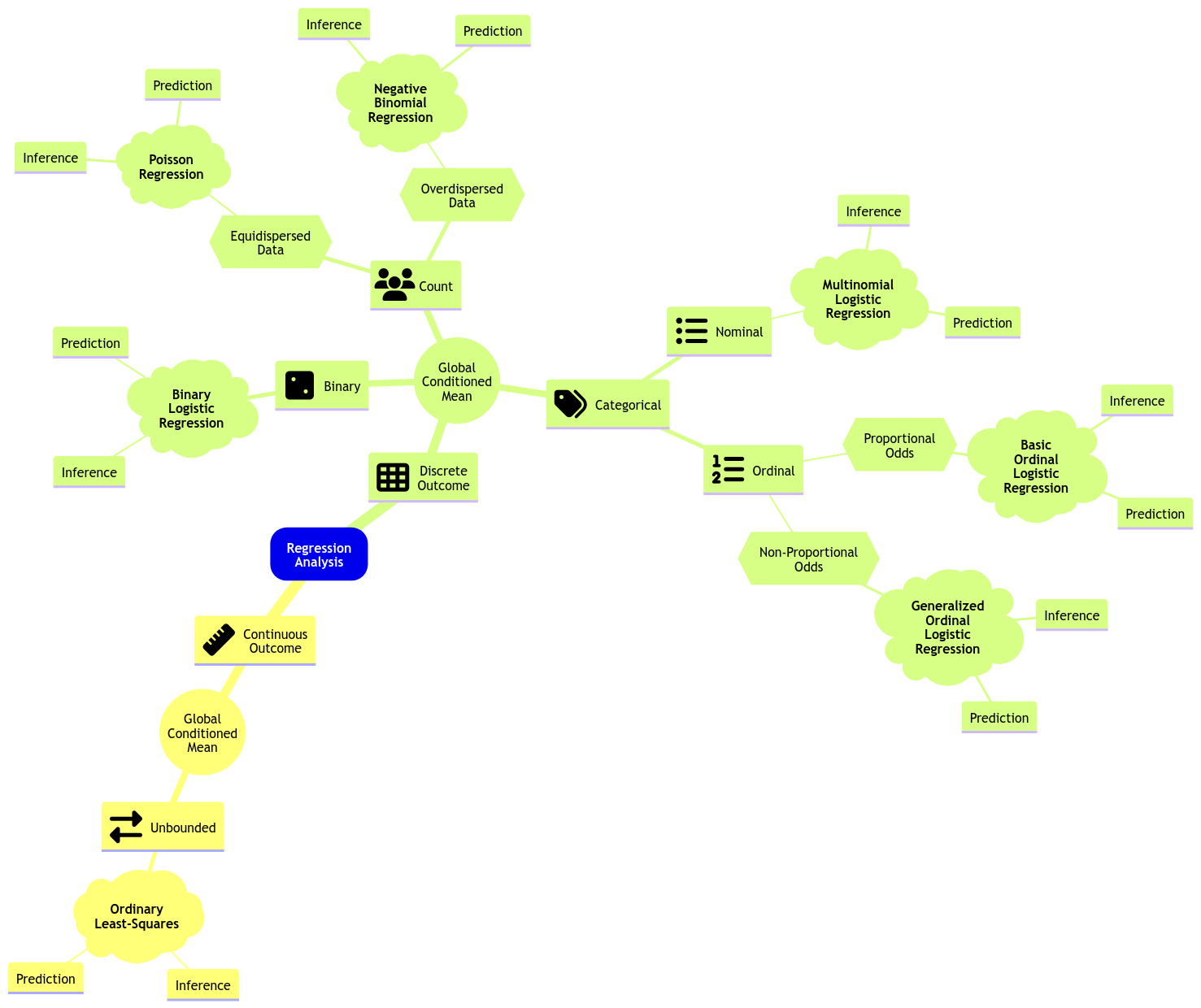
Therefore, the ideal approach is an alternative logistic regression that suits ordinal responses. Hence, the existence of the Ordinal Logistic regression model. Let us expand the regression mindmap as in Figure 1 to include this new model. Note there is a key characteristic called proportional odds, which is reflected in the data modelling framework and to be discussed today.

4 College Juniors Dataset

To illustrate the use of this generalized linear model (GLM), let us introduce an adequate dataset.

The College Juniors Dataset

The data frame college_data was obtained from the webpage of the UCLA Statistical Consulting Group. This dataset contains the results of a survey applied to \(n = 400\) college juniors regarding the factors that influence their decision to apply to graduate school.

The dataset contains the following variables:

decision: how likely the student will apply to graduate school, a discrete and ordinal response with three increasing categories (unlikely, somewhat likely, and very likely).
parent_ed: whether at least one parent has a graduate degree, a discrete and binary explanatory variable (Yes and No).
GPA: the student’s current GPA, a continuous explanatory variable.

Important

In this example, variable decision will be our response of interest. However, before proceeding with our regression analysis. Let us set it up as an ordered factor via function as.ordered().

Main Statistical Inquiries

Let us suppose we want to assess the following:

Is decision statistically related to parent_ed and GPA?
How can we interpret these statistical relationships (if there are any!)?

5 Exploratory Data Analysis

Let us plot the data first. Since decision is a discrete and ordinal response, we have to be careful about the class of plots we are using regarding exploratory data analysis (EDA).

To explore visually the relationship between decision and GPA , we will use the following side-by-side plots:

Boxplots.
Violin plots.

The code below creates side-by-side boxplots and violin plots, where GPA is on the \(y\)-axis, and all categories of decision are on the \(x\)-axis. The side-by-side violin plots show the mean of GPA by decision category in red points.

Now, how can we visually explore the relationship between decision and parent_ed?

In the case of two categorical explanatory variables, we can use stacked bar charts. Each bar will show the percentages (depicted on the \(y\)-axis) of college students falling on each ordered category of decision with the categories found in parent_ed on the \(x\)-axis. This class of bars will allow us to compare both levels of parent_ed in terms of the categories of decision.

First of all, we need to do some data wrangling. The code below obtains the proportions for each level of decision conditioned on the categories of parent_ed. If we add up all proportions corresponding to No or Yes, we will obtain 1.

Then, we code the corresponding plot:

Exercise 9

What can we see descriptively from the above plots?

6 Data Modelling Framework

Let us suppose that a given discrete ordinal response \(Y_i\) (for \(i = 1, \dots, n\)) has categories \(1, 2, \dots, m\) in a training set of size \(n\).

Important

Categories \(1, 2, \dots, m\) implicate an ordinal scale here, i.e., \(1 < 2 < \dots < m\).

Also, note there is more than one class of Ordinal Logistic regression. We will review the proportional odds version, which is also a cumulative logit model.

We set up the Ordinal Logistic regression model for this specific dataset with \(m = 3\). For the \(i\)th observation with the continuous \(X_{i, \texttt{GPA}}\) and the dummy variable

\[ X_{i, \texttt{parent\_ed}} = \begin{cases} 1 \; \; \; \; \mbox{at least one parent has a graduate degree},\\ 0 \; \; \; \; \mbox{neither of the parents has a graduate degree;} \end{cases} \]

the model will indicate how each one of the regressors affects the cumulative logarithm of the odds in decision for the following \(2\) situations:

\[ \begin{gather*} \text{Level } \texttt{somewhat likely} \text{ or any lesser degree versus level } \texttt{very likely} \\ \text{Level } \texttt{unlikely} \text{ versus level } \texttt{somewhat likely} \text{ or any higher degree} \end{gather*} \]

Then, we have the following system of \(2\) equations:

\[ \begin{align*} \eta_i^{(\texttt{somewhat likely})} &= \log\left[\frac{P(Y_i \leq \texttt{somewhat likely} \mid X_{i, \texttt{GPA}},X_{i, \texttt{parent\_ed}})}{P(Y_i = \texttt{very likely} \mid X_{i, \texttt{GPA}}, X_{i, \texttt{parent\_ed}})}\right] \\ &= \beta_0^{(\texttt{somewhat likely})} - \beta_1 X_{i, \texttt{GPA}} - \beta_2 X_{i, \texttt{parent\_ed}} \end{align*} \tag{1}\]

\[ \begin{align*} \eta_i^{(\texttt{unlikely})} &= \log\left[\frac{P(Y_i = \texttt{unlikely} \mid X_{i, \texttt{GPA}},X_{i, \texttt{parent\_ed}})}{P(Y_i \geq \texttt{somewhat likely} \mid X_{i, \texttt{GPA}},X_{i, \texttt{parent\_ed}})}\right] \\ &= \beta_0^{(\texttt{unlikely})} - \beta_1 X_{i, \texttt{GPA}} - \beta_2 X_{i, \texttt{parent\_ed}}. \end{align*} \tag{2}\]

The system has \(2\) intercepts but only \(2\) regression coefficients. Check the signs of the common \(\beta_1\) and \(\beta_2\), which are minuses. This is a fundamental parameterization of the proportional odds model.

To make coefficient intepretation easier, we could re-expresss the equations of \(\eta_i^{(\texttt{somewhat likely})}\) (i.e., Equation 1) and \(\eta_i^{(\texttt{unlikely})}\) (i.e., Equation 2) as follows:

\[ \begin{align*} \frac{P(Y_i = \texttt{very likely} \mid X_{i, \texttt{GPA}},X_{i, \texttt{parent\_ed}})}{P(Y_i \leq \texttt{somewhat likely} \mid X_{i, \texttt{GPA}},X_{i, \texttt{parent\_ed}})} &= \exp\big(-\beta_0^{(\texttt{somewhat likely})}\big) \times \\ & \qquad \exp\big(\beta_1 X_{i, \texttt{GPA}}\big) \times \\ & \qquad \quad \exp\big(\beta_2 X_{i, \texttt{parent\_ed}}\big) \end{align*} \]

\[ \begin{align*} \frac{P(Y_i \geq \texttt{somewhat likely} \mid X_{i, \texttt{GPA}},X_{i, \texttt{parent\_ed}})}{P(Y_i = \texttt{unlikely} \mid X_{i, \texttt{GPA}},X_{i, \texttt{parent\_ed}})} &= \exp\big(-\beta_0^{(\texttt{unlikely})}\big) \times \\ & \qquad \exp\big(\beta_1 X_{i, \texttt{GPA}}\big) \times \\ & \qquad \quad \exp\big(\beta_2 X_{i, \texttt{parent\_ed}}\big). \end{align*} \]

Both regression coefficients (\(\beta_1\) and \(\beta_2\)) have a multiplicative effect on the odds on the left-hand side. Moreover, given the proportional odds assumptions, these rregression coefficients are the same for both cumulative odds.

6.1 What is the math for the general case with \(m\) response categories and \(k\) regressors?

Before going into the model’s mathematical notation in general, we have to point out that Ordinal Logistic regression will indicate how each one of the \(k\) regressors \(X_{i,1}, \dots, X_{i,k}\) affects the cumulative logarithm of the odds in the ordinal response for the following \(m - 1\) situations:

\[ \begin{gather*} \text{Level } m - 1 \text{ or any lesser degree versus level } m\\ \text{Level } m - 2 \text{ or any lesser degree versus level } m - 1 \text{ or any higher degree}\\ \vdots \\ \text{Level } 2 \text{ or any lesser degree versus level } 3 \text{ or any higher degree}\\ \text{Level } 1 \text{ versus level } 2 \text{ or any higher degree}\\ \end{gather*} \]

These \(m - 1\) situations are translated into cumulative probabilities using the logarithms of the odds on the left-hand side (\(m - 1\) link functions) subject to the linear combination of the \(k\) regressors \(X_{i,j}\) (for \(j = 1, \dots, k\)):

\[ \begin{gather*} \eta_i^{(m - 1)} = \log\left[\frac{P(Y_i \leq m - 1 \mid X_{i,1}, \ldots, X_{i,k})}{P(Y_i = m \mid X_{i,1}, \ldots, X_{i,k})}\right] = \beta_0^{(m - 1)} - \beta_1 X_{i, 1} - \ldots - \beta_k X_{i, k} \\ \eta_i^{(m - 2)} = \log\left[\frac{P(Y_i \leq m - 2 \mid X_{i,1}, \ldots, X_{i,k})}{P(Y_i > m - 2 \mid X_{i,1}, \ldots, X_{i,k})}\right] = \beta_0^{(m - 2)} - \beta_1 X_{i, 1} - \ldots - \beta_k X_{i, k} \\ \vdots \\ \eta_i^{(2)} = \log\left[\frac{P(Y_i \leq 2 \mid X_{i,1}, \ldots, X_{i,k})}{P(Y_i > 2 \mid X_{i,1}, \ldots, X_{i,k})}\right] = \beta_0^{(2)} - \beta_1 X_{i, 1} - \ldots - \beta_k X_{i, k} \\ \eta_i^{(1)} = \log\left[\frac{P(Y_i = 1 \mid X_{i,1}, \ldots, X_{i,k})}{P(Y_i > 1 \mid X_{i,1}, \ldots, X_{i,k})}\right] = \beta_0^{(1)} - \beta_1 X_{i, 1} - \ldots - \beta_k X_{i, k}. \end{gather*} \tag{3}\]

Note that the system above has \(m - 1\) intercepts but only \(k\) regression coefficients. In general, the previous \(m - 1\) equations can be generalized for levels \(j = m - 1, \dots, 1\) as follows:

\[ \begin{gather*} \eta_i^{(j)} = \log\left[\frac{P(Y_i \leq j \mid X_{i,1}, \ldots, X_{i,k})}{P(Y_i > j \mid X_{i,1}, \ldots, X_{i,k})}\right] = \beta_0^{(j)} - \beta_1 X_{i, 1} - \beta_2 X_{i, 2} - \ldots - \beta_k X_{i, k} \\ \; \; \; \; \; \; \; \; \Rightarrow \; P(Y_i \leq j \mid X_{i,1}, \ldots, X_{i,k}) = \frac{\exp\left(\beta_0^{(j)} - \beta_1 X_{i, 1} - \beta_2 X_{i, 2} - \ldots - \beta_k X_{i, k}\right)}{1 + \exp\left(\beta_0^{(j)} - \beta_1 X_{i, 1} - \beta_2 X_{i, 2} - \ldots - \beta_k X_{i, k}\right)}. \end{gather*} \]

The probability that \(Y_i\) will fall in the category \(j\) can be computed as follows:

\[ \begin{align*} p_{i,j} &= P(Y_i = j \mid X_{i,1}, \ldots, X_{i,k}) \\ &= P(Y_i \leq j \mid X_{i,1}, \ldots, X_{i,k}) - P(Y_i \leq j - 1 \mid X_{i,1}, \ldots, X_{i,k}), \end{align*} \]

which leads to

\[ P(Y_i = 1) = p_{i,1} \;\;\;\; P(Y_i = 2) = p_{i,2} \;\; \dots \;\; P(Y_i = m) = p_{i,m} \]

where

\[ \sum_{j = 1}^m p_{i,j} = p_{i,1} + p_{i,2} + \dots + p_{i,m} = 1. \]

Now, let us check the next in-class question via iClicker.

Exercise 10

Suppose we have a case with an ordered response of five levels and four continuous regressors; how many link functions, intercepts, and coefficients will our Ordinal Logistic regression model have under a proportional odds assumption?

A. Four link functions, four intercepts, and sixteen regression coefficients.

B. Five link functions, five intercepts, and five regression coefficients.

C. Five link functions, five intercepts, and twenty regression coefficients.

D. Four link functions, four intercepts, and four regression coefficients.

6.2 (Optional) Mathematically, what does the proportional odds assumption stand for?

Let us show mathematically what the proportional odds assumption stand for in Ordinal Logistic regression for the general case of a discrete ordinal response \(Y_i\) (for \(i = 1, \dots, n\)) with categories \(1, 2, \dots, m\) in a training set of size \(n\), subject to \(k\) regressors \(X_{i,1}, \dots, X_{i,k}\). Recall these \(m\) categories implicate an ordinal scale, i.e., \(1 < 2 < \dots < m\).

The cumulative logarithm of the odds system in 3 can be rearranged as follows using exponentiation:

\[ \begin{gather*} \frac{P(Y_i \leq m - 1 \mid X_{i,1}, \ldots, X_{i,k})}{P(Y_i = m \mid X_{i,1}, \ldots, X_{i,k})} = \exp \left( \beta_0^{(m - 1)} - \beta_1 X_{i, 1} - \ldots - \beta_k X_{i, k} \right) \\ \frac{P(Y_i \leq m - 2 \mid X_{i,1}, \ldots, X_{i,k})}{P(Y_i > m - 2 \mid X_{i,1}, \ldots, X_{i,k})} = \exp \left( \beta_0^{(m - 2)} - \beta_1 X_{i, 1} - \ldots - \beta_k X_{i, k} \right) \\ \vdots \\ \frac{P(Y_i \leq 2 \mid X_{i,1}, \ldots, X_{i,k})}{P(Y_i > 2 \mid X_{i,1}, \ldots, X_{i,k})} = \exp \left( \beta_0^{(2)} - \beta_1 X_{i, 1} - \ldots - \beta_k X_{i, k} \right) \\ \frac{P(Y_i = 1 \mid X_{i,1}, \ldots, X_{i,k})}{P(Y_i > 1 \mid X_{i,1}, \ldots, X_{i,k})} = \exp \left( \beta_0^{(1)} - \beta_1 X_{i, 1} - \ldots - \beta_k X_{i, k} \right). \end{gather*} \]

Then, we apply the exponent laws on the righ-hand side of the system:

\[ \begin{gather*} \frac{P(Y_i \leq m - 1 \mid X_{i,1}, \ldots, X_{i,k})}{P(Y_i = m \mid X_{i,1}, \ldots, X_{i,k})} = \exp \left( \beta_0^{(m - 1)} \right) \exp \left( - \beta_1 X_{i, 1} - \ldots - \beta_k X_{i, k} \right) \\ \frac{P(Y_i \leq m - 2 \mid X_{i,1}, \ldots, X_{i,k})}{P(Y_i > m - 2 \mid X_{i,1}, \ldots, X_{i,k})} = \exp \left( \beta_0^{(m - 2)} \right) \exp \left( - \beta_1 X_{i, 1} - \ldots - \beta_k X_{i, k} \right) \\ \vdots \\ \frac{P(Y_i \leq 2 \mid X_{i,1}, \ldots, X_{i,k})}{P(Y_i > 2 \mid X_{i,1}, \ldots, X_{i,k})} = \exp \left( \beta_0^{(2)} \right) \exp \left( - \beta_1 X_{i, 1} - \ldots - \beta_k X_{i, k} \right) \\ \frac{P(Y_i = 1 \mid X_{i,1}, \ldots, X_{i,k})}{P(Y_i > 1 \mid X_{i,1}, \ldots, X_{i,k})} = \exp \left( \beta_0^{(1)} \right) \exp \left( - \beta_1 X_{i, 1} - \ldots - \beta_k X_{i, k} \right). \end{gather*} \]

The above right-hand side can be isolated as follows:

\[ \begin{gather*} \exp \left( - \beta_0^{(m - 1)} \right) \frac{P(Y_i \leq m - 1 \mid X_{i,1}, \ldots, X_{i,k})}{P(Y_i = m \mid X_{i,1}, \ldots, X_{i,k})} = \exp \left( - \beta_1 X_{i, 1} - \ldots - \beta_k X_{i, k} \right) \\ \exp \left( - \beta_0^{(m - 2)} \right) \frac{P(Y_i \leq m - 2 \mid X_{i,1}, \ldots, X_{i,k})}{P(Y_i > m - 2 \mid X_{i,1}, \ldots, X_{i,k})} = \exp \left( - \beta_1 X_{i, 1} - \ldots - \beta_k X_{i, k} \right) \\ \vdots \\ \exp \left( - \beta_0^{(2)} \right) \frac{P(Y_i \leq 2 \mid X_{i,1}, \ldots, X_{i,k})}{P(Y_i > 2 \mid X_{i,1}, \ldots, X_{i,k})} = \exp \left( - \beta_1 X_{i, 1} - \ldots - \beta_k X_{i, k} \right) \\ \exp \left( - \beta_0^{(1)} \right) \frac{P(Y_i = 1 \mid X_{i,1}, \ldots, X_{i,k})}{P(Y_i > 1 \mid X_{i,1}, \ldots, X_{i,k})} = \exp \left( - \beta_1 X_{i, 1} - \ldots - \beta_k X_{i, k} \right). \end{gather*} \]

This above rearranged system has the same elements on the right-hand side, which allows us to summarize their left-hand side as:

\[ \begin{gather*} \exp{\left(-\beta_0^{(m - 1)}\right)} \frac{P(Y_i \leq m - 1 \mid X_{i,1}, \ldots, X_{i,k})}{P(Y_i = m \mid X_{i,1}, \ldots, X_{i,k})} = \dots = \exp{\left(-\beta_0^{(1)}\right)} \frac{\Pr(Y_i = 1 \mid X_{i,1}, \ldots, X_{i,k})}{\Pr(Y_i > 1 \mid X_{i,1}, \ldots, X_{i,k})}. \end{gather*} \]

Finally, these are the proportional odds:

\[ \begin{gather*} \frac{P(Y_i \leq m - 1 \mid X_{i,1}, \ldots, X_{i,k})}{P(Y_i = m \mid X_{i,1}, \ldots, X_{i,k})} \propto \dots \propto \frac{P(Y_i = 1 \mid X_{i,1}, \ldots, X_{i,k})}{P(Y_i > 1 \mid X_{i,1}, \ldots, X_{i,k})}. \end{gather*} \tag{4}\]

Important

Note the symbol \(\propto\) indicates “proportional to” in Equation 4.

The proportional odds assumption says that our \(k\) regressors have the same directional effect and the same strength no matter where we draw the line between “lower” and “higher” categories of the ordinal response.

Concretely, Ordinal Logistic regression looks at several “splits” of the response, like \(Y = 1\) versus \(Y > 1\), \(Y \leq 2\) versus \(Y > 2\), and so on. Proportional odds assumes that when a given regressor increases by one unit, it multiplies the odds of being in a higher category (rather than at or below the cutoff) by the same factor for every cutoff. The cutoffs themselves can shift (each cutoff has its own baseline, i.e., regression intercept), but each one of the \(k\) regression coefficients does not change across cutoffs.

6.3 A Graphical Intuition of the Proportional Odds Assumption

The previous section showed mathematically what the proportional odds assumption stands for in the Ordinal Logistic regression model with \(k\) regressors and a training set of size \(n\), using a response of \(m\) levels in general. In plain terms, we just showed that regressors “push” observations up or down the ordinal response scale in a consistent way, rather than having different effects at different parts of the scale.

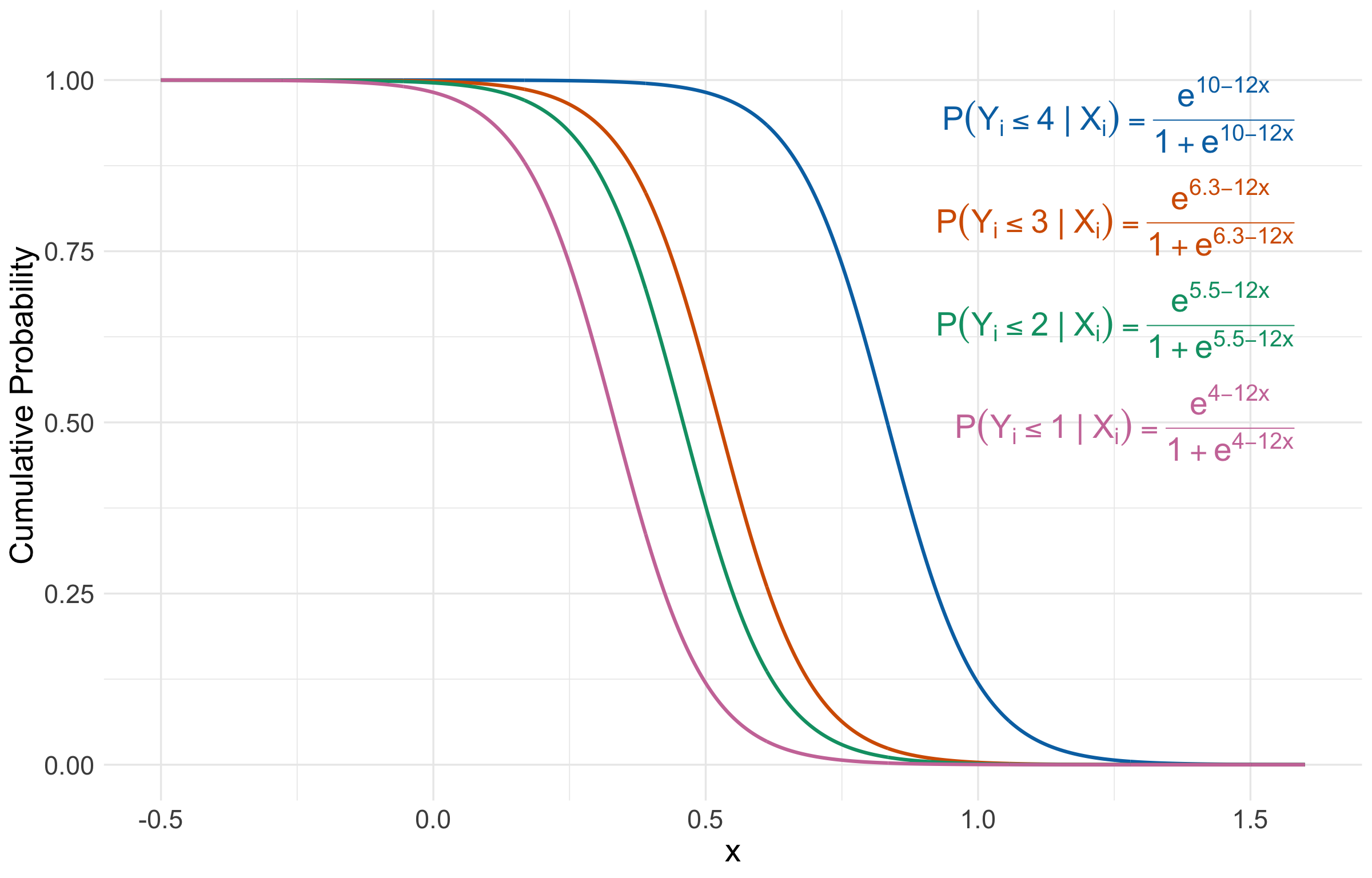
That said, let us show the graphical intuition of this assumption with an example of an ordinal response of \(5\) levels and a single continuous regressor \(X_{i , 1}\) (which is assumed to be unbounded!) with \(i = 1, \dots, n\) for a training set of size \(n\). The system of cumulative logit equations is the following:

\[ \begin{gather*} \eta_i^{(4)} = \log\left[\frac{P(Y_i \leq 4 \mid X_{i,1})}{P(Y_i = 5 \mid X_{i,1})}\right] = \beta_0^{(4)} - \beta_1 X_{i, 1} \\ \eta_i^{(3)} = \log\left[\frac{P(Y_i \leq 3 \mid X_{i,1})}{P(Y_i > 3 \mid X_{i,1})}\right] = \beta_0^{(3)} - \beta_1 X_{i, 1} \\ \eta_i^{(2)} = \log\left[\frac{P(Y_i \leq 2 \mid X_{i,1})}{P(Y_i > 2 \mid X_{i,1})}\right] = \beta_0^{(2)} - \beta_1 X_{i, 1} \\ \eta_i^{(1)} = \log\left[\frac{P(Y_i = 1 \mid X_{i,1})}{P(Y_i > 1 \mid X_{i,1})}\right] = \beta_0^{(1)} - \beta_1 X_{i, 1}. \end{gather*} \]

This above system could be mathematically expressed as follows:

\[ \begin{gather*} P(Y_i \leq 4 \mid X_{i,1}) = \frac{\exp\left(\beta_0^{(4)} - \beta_1 X_{i, 1} \right)}{1 + \exp\left(\beta_0^{(4)} - \beta_1 X_{i, 1}\right)} \\ P(Y_i \leq 3 \mid X_{i,1}) = \frac{\exp\left(\beta_0^{(3)} - \beta_1 X_{i, 1} \right)}{1 + \exp\left(\beta_0^{(3)} - \beta_1 X_{i, 1}\right)} \\ P(Y_i \leq 2 \mid X_{i,1}) = \frac{\exp\left(\beta_0^{(2)} - \beta_1 X_{i, 1} \right)}{1 + \exp\left(\beta_0^{(2)} - \beta_1 X_{i, 1}\right)} \\ P(Y_i \leq 1 \mid X_{i,1}) = \frac{\exp\left(\beta_0^{(1)} - \beta_1 X_{i, 1} \right)}{1 + \exp\left(\beta_0^{(1)} - \beta_1 X_{i, 1}\right)}. \\ \end{gather*} \tag{5}\]

Note we have four intercepts \((\beta_0^{(1)}, \beta_0^{(2)}, \beta_0^{(3)}, \beta_0^{(4)})\) and a single coefficient \(\beta_1\). Moreover, let us assume we estimate these five parameters to be the following:

\[ \begin{gather*} \hat{\beta}_0^{(1)} = 4\\ \hat{\beta}_0^{(2)} = 5.5 \\ \hat{\beta}_0^{(3)} = 6.3 \\ \hat{\beta}_0^{(4)} = 10 \\ \hat{\beta}_1 = 12. \end{gather*} \]

Let us check our estimated sigmoid functions! Figure 2 shows the four estimated logistic (\(S\)-shaped) curves of the form \(P(Y_i \leq u \mid X_{i,1})\) for \(u = 1, 2, 3, 4\) depicted in the system shown in 5. Each curve is a cumulative probability (i.e., the \(y\)-axis): for a given value of \(X_{i,1}\), it tells you the probability that the ordinal outcome falls at or below category \(u\). Because the curves are decreasing here, larger values of \(X_{i,1}\) make it less probable that \(Y_i\) is in the lower categories; equivalently, they shift probability mass toward higher categories.

The curves are separated horizontally because each cutoff \(u = 1, 2, 3, 4\) has its own threshold (i.e., intercept): higher cutoffs sit further to the right on the \(x\)-axis since it is easier to be \(\leq 4\) than \(\leq 1\) as \(X_{i,1}\) gets more positive. What ties them together is the proportional odds assumption: all four curves have the same estimated coefficient \(\hat{\beta}_1 = 12\) (i.e., they are parallel shifts of one another). In plain words, the proportional odds assumption says the effect of \(X_{i,1}\) is consistent across all cutpoints: a one-unit increase in \(X_{i,1}\) changes the odds of being in a higher category by the same multiplicative factor, no matter whether you are comparing “\(\leq 1\) versus \(>1\)”, “\(\leq 2\) vs \(>2\)”, and so on.

Figure 2: Sigmoid functions under a proportional odds assumption.

7 Estimation

All parameters in the Ordinal Logistic regression model are also unknown. Therefore, model estimates are obtained through maximum likelihood, where we also assume a Multinomial joint probability mass function of the \(n\) responses \(Y_i\). Moreover, this Multinomial assumption plays around with cumulative probabilities in the joint likelihood function as discussed in Agresti (2013) in Chapter 8 (Section 8.2.2).

To fit the model with the package MASS, we use the function polr(), which obtains the corresponding estimates. The argument Hess = TRUE is required to compute the Hessian matrix of the log-likelihood function, which is used to obtain the standard errors of the estimates.

Important

Maximum likelihood estimation in this regression model is quite complex compared to the challenging Exercise 5 in lab1. Thus, the proof will be out of the scope of this course.

Note

If you would like to check a further rationale on the use of the Hessian matrix to obtain the standard errors of regression estimates, you can find good insights into this matter via the classical linear regression model (i.e., Ordinary Least-squares but in its maximum likelihood estimation flavour) in this resource.

8 Inference

We can determine whether a regressor is statistically associated with the logarithm of the cumulative odds through hypothesis testing for the parameters \(\beta_j\). We also use the Wald statistic \(z_j\):

\[ z_j = \frac{\hat{\beta}_j}{\mbox{se}(\hat{\beta}_j)} \]

to test the hypotheses

\[ \begin{gather*} H_0: \beta_j = 0\\ H_a: \beta_j \neq 0. \end{gather*} \]

The null hypothesis \(H_0\) indicates that the \(j\)th regressor associated to \(\beta_j\) does not affect the response variable in the model, and the alternative hypothesis \(H_a\) otherwise. Moreover, provided the sample size \(n\) is large enough, \(z_j\) has an approximately Standard Normal distribution under \(H_0\).

R provides the corresponding \(p\)-values for each \(\beta_j\). The smaller the \(p\)-value, the stronger the evidence against the null hypothesis \(H_0\). As in the previous regression models, we would set a predetermined significance level \(\alpha\) (usually taken to be 0.05) to infer if the \(p\)-value is small enough. If the \(p\)-value is smaller than the predetermined level \(\alpha\), then you could claim that there is evidence to reject the null hypothesis. Hence, \(p\)-values that are small enough indicate that the data provides evidence in favour of association (or causation in the case of an experimental study!) between the response variable and the \(j\)th regressor.

Furthermore, given a specified level of confidence where \(\alpha\) is the significance level, we can construct approximate \((1 - \alpha) \times 100\%\) confidence intervals for the corresponding true value of \(\beta_j\):

\[ \hat{\beta}_j \pm z_{\alpha/2}\mbox{se}(\hat{\beta}_j), \]

where \(z_{\alpha/2}\) is the upper \(\alpha/2\) quantile of the Standard Normal distribution.

Function polr() does not provide \(p\)-values, but we can compute them as follows:

Terms unlikely|somewhat likely and somewhat likely|very likely refer to the estimated intercepts \(\hat{\beta}_0^{(\texttt{unlikely})}\) and \(\hat{\beta}_0^{(\texttt{somewhat likely})}\), respectively (note the hat notation).

Finally, we see that those coefficients associated with GPA and parent_ed are statistically significant with \(\alpha = 0.05\). Function confint() can provide the 95% confidence intervals for the estimates contained in tidy().

9 Coefficient Interpretation

The interpretation of the Ordinal Logistic regression coefficients will change since we are modelling cumulative probabilities. Let us interpret the association of decision with GPA and parent_ed.

By using the column exp.estimate, along with the model equations on the original scale of the cumulative odds, we interpret the two regression coefficients above by each odds as follows:

For the odds

\(\beta_1\): “for each one-unit increase in the GPA, the odds that the student is very likely versus somewhat likely or unlikely to apply to graduate school increase by \(\exp \left( \hat{\beta}_1 \right) = 1.82\) times (while holding parent_ed constant).”

\(\beta_2\): “for those respondents whose parents attended to graduate school, the odds that the student is very likely versus somewhat likely or unlikely to apply to graduate school increase by \(\exp \left( \hat{\beta}_2 \right) = 2.86\) times (when compared to those respondents whose parents did not attend to graduate school and holding GPA constant).”

For the odds

\(\beta_1\): “for each one-unit increase in the GPA, the odds that the student is very likely or somewhat likely versus unlikely to apply to graduate school increase by \(\exp \left( \hat{\beta}_1 \right) = 1.82\) times (while holding parent_ed constant).”

\(\beta_2\): “for those respondents whose parents attended to graduate school, the odds that the student is very likely or somewhat likely versus unlikely to apply to graduate school increase by \(\exp \left( \hat{\beta}_2 \right) = 2.86\) times (when compared to those respondents whose parents did not attend to graduate school and holding GPA constant).”

10 Predictions

Aside from our main statistical inquiries, using the function predict() with the object ordinal_model, we can obtain the estimated probabilities to apply to graduate school (associated to unlikely, somewhat likely, and very likely) for a student with a GPA of 3.5 whose parents attended to graduate school.

We can see that it is somewhat likely to apply to graduate school with a probability of 0.48. Thus, we could classify the student in this ordinal category.

(Optional) Predicting Cumulative Odds

Beside predicting probabilities for each ordinal response category, we can predict the corresponding cumulative odds. Unfortunately, predict() with polr() does not provide a quick way to compute this model’s corresponding predicted cumulative odds for a new observation. Nonetheless, we could use function vglm()(from package VGAM) while keeping in mind that this function labels the response categories as numbers. Let us check this for decision with levels().

Hence, unlikely is 1, somewhat likely is 2, and very likely is 3. Now, let us use vglm() with propodds to fit the same model (named ordinal_model_vglm) as follows:

We will double-check whether ordinal_model_vglm provides the same classification probabilities via predict(). Note that the function parameterization changes to type = "response".

Yes, we get identical results using vglm(). Now, let us use predict() with ordinal_model_vglm to obtain the predicted cumulative odds for a student with a GPA of 3.5 whose parents attended to graduate school (via argument type = "link" in predict()).

Then, let us take these predictions to the odds’ original scale via exp().

Again, we see the numeric labels (a drawback of using vglm()). We interpret these predictions as follows:

\(\frac{P(Y_i = \texttt{very likely} \mid X_{i, \texttt{GPA}},X_{i, \texttt{parent\_ed}})}{P(Y_i \leq \texttt{somewhat likely} \mid X_{i, \texttt{GPA}},X_{i, \texttt{parent\_ed}})}\), i.e., P[Y>=3] (label 3, very likely): “a student, with a GPA of 3.5 whose parents attended to graduate school, is 3.03 (\(1 / 0.33\)) times somewhat likely or unlikely versus very likely to apply to graduate school.” This prediction goes in line with the predicted probabilities above, given that somewhat likely has a probability of 0.48 and unlikely a probability of 0.27.
\(\frac{P(Y_i \geq \texttt{somewhat likely} \mid X_{i, \texttt{GPA}},X_{i, \texttt{parent\_ed}})}{P(Y_i = \texttt{unlikely} \mid X_{i, \texttt{GPA}},X_{i, \texttt{parent\_ed}})}\), i.e., P[Y>=2] (label 2, somewhat likely): “a student, with a GPA of 3.5 whose parents attended to graduate school, is 2.68 times very likely or somewhat likely versus unlikely to apply to graduate school.” This prediction goes in line with the predicted probabilities above, given that somewhat likely has a probability of 0.48 and very likely a probability of 0.25.

11 Model Selection

To perform model selection, we can use the same techniques from lecture2. That said, some R coding functions might not be entirely available for the polr() models. Still, these statistical techniques and metrics can be manually coded.

12 Non-proportional Odds

Now, we might wonder

What happens if we do not fulfil the proportional odds assumption in our Ordinal Logistic regression model?

12.1 The Brant-Wald Test

It is essential to remember that the Ordinal Logistic model under the proportional odds assumption is the first step when performing Regression Analysis on an ordinal response.

Once this model has been fitted, it is possible to assess whether it fulfils this strong assumption statistically.

We can do it via the Brant-Wald test:

This tool statistically assesses whether our model globally fulfils this assumption. It has the following hypotheses:

\[ \begin{gather*} H_0:\ \text{Our Ordinal Logistic regression model globally fulfils} \\ \text{the proportional odds assumption.} \\ H_a:\ \text{Otherwise.} \end{gather*} \]

Moreover, it also performs further hypothesis testing on each regressor. With \(k\) regressors for \(j = 1, \dots, k\); we have the following hypotheses:

\[ \begin{gather*} H_0:\ \text{The } j \text{th regressor in our Ordinal Logistic regression model fulfils} \\ \text{the proportional odds assumption.} \\ H_a:\ \text{Otherwise.} \end{gather*} \]

Function brant() from package brant implements this tool, which can be used in our polr() object ordinal_model:

The row Omnibus represents the global model, while the other two rows correspond to our two regressors: parent_ed and GPA. Note that with \(\alpha = 0.05\), we are completely fulfilling the proportional odds assumption (the column probability delivers the corresponding \(p\)-values).

Important

The Brant Wald test essentially compares this basic Ordinal Logistic regression model of \(m - 1\) cumulative logit functions (i.e., the ordinal response has \(m\) categories) versus a combination of \(m − 1\) correlated Binary Logistic regressions.

12.2 A Non-proportional Odds Model

Suppose that our example case does not fulfil the proportional odds assumption according to the Brant Wald test. It is possible to have a model under a non-proportional odds assumption as follows:

\[ \begin{align*} \eta_i^{(\texttt{somewhat likely})} &= \log\left[\frac{P(Y_i \leq \texttt{somewhat likely} \mid X_{i, \texttt{GPA}},X_{i, \texttt{parent\_ed}})}{P(Y_i = \texttt{very likely} \mid X_{i, \texttt{GPA}}, X_{i, \texttt{parent\_ed}})}\right] \\ &= \beta_0^{(\texttt{somewhat likely})} - \beta_1^{(\texttt{somewhat likely})} X_{i, \texttt{GPA}} - \beta_2^{(\texttt{somewhat likely})} X_{i, \texttt{parent\_ed}} \end{align*} \]

\[ \begin{align*} \eta_i^{(\texttt{unlikely})} &= \log\left[\frac{P(Y_i = \texttt{unlikely} \mid X_{i, \texttt{GPA}},X_{i, \texttt{parent\_ed}})}{P(Y_i \geq \texttt{somewhat likely} \mid X_{i, \texttt{GPA}},X_{i, \texttt{parent\_ed}})}\right] \\ &= \beta_0^{(\texttt{unlikely})} - \beta_1^{(\texttt{unlikely})} X_{i, \texttt{GPA}} - \beta_2^{(\texttt{unlikely})} X_{i, \texttt{parent\_ed}}. \end{align*} \]

This is called a Generalized Ordinal Logistic regression model. This class of models can be fit via the function cumulative() from package VGAM. Note that estimation, inference, coefficient interpretation, and predictions are conducted in a similar way compared to the proportional odds model.

Exercise 11

Why would we have to be cautious when fitting a non-proportional odds model in the context of a response with a considerable number of ordinal levels and regressors?

13 Wrapping Up on Categorical Regression Models

Multinomial and Ordinal Logistic regression models address cases where our response is discrete and categorical. These models are another class GLMs with their corresponding link functions.
Multinomial Logistic regression approaches nominal responses. It heavily relies on a baseline response level and the odds’ natural logarithm.
Ordinal Logistic regression approaches ordinal responses. It relies on cumulative odds on an ordinal scale.
We have to be careful with coefficient interpretations in these models, especially with the cumulative odds. This will imply an effective communication of these estimated models for inferential matters.