Lecture 8 - Missing Data

Today’s Learning Goals

By the end of this lecture, you should be able to:

• Identify and explain the three common types of missing data mechanisms.

• Identify a potential consequence of removing missing data on downstream analyses.

• Identify a potential consequence of a mean imputation method on downstream analyses.

• Identify the four steps involved with a multiple imputation method for handling missing data.

• Use the mice package in R to fit multiple imputed models.

Loading Libraries

options(repr.matrix.max.rows = 20)
library(tidyverse)
library(nycflights13)
library(mice)

1. Types of Missing Data

In Statistics, there are three types of missing data:

• Missing completely at random (MCAR).

• Missing at random (MAR).

• Missing not at random (MNAR).

It is in our best interest to identify the type of missing data we have. Proper identification will determine the class of approach we will take to deal with missingness in any statistical analysis.

1.1. Missing Completely At Random (MCAR)

In this type, missing data appear totally by chance. Hence, missingness is independent of the data. Roughly speaking, all our observations (rows in the dataset) have the same chance of containing missing data (i.e., an NA in one of the columns).

Important

It is the ideal class of missing data since there is no missingness pattern.

Example

We are trying to count the number of car accidents in Vancouver. To do that, we are monitoring the traffic in 100 strategic points of the city with cameras. Say that we count how many vehicles passed by each one of those cameras for every minute of the day. We have 101 variables: time, Camera_1, …, Camera_100.

Suppose that any camera has a \(1\%\) chance of failing for any given minute. If a camera fails, you get MCAR data for that minute.

1.2. Missing At Random (MAR)

In this type, missingness depends on the observed data we have. Therefore, we could use some imputation techniques for this missingness, such as multiple imputation (to be covered later on today), based on the rest of our available data (a hot deck imputation technique).

Important

Missing data imputation techniques are divided into two classes:

• Hot deck: Those incomplete rows in our current dataset are imputed using the information provided by the complete rows within the same dataset.

• Cold deck: Those incomplete rows in our current dataset are imputed using the information provided by the complete rows of another dataset with the same column structure.

The scope of this lecture pertains to hot deck techniques.

Example

Following up with the previous example, an external device is attached to the cameras to increase the image quality at low light situations (night time) and we have the recording time in our dataset. The external device is activated from 6 p.m. to 5 a.m. However, the device has a \(10\%\) chance of not working in a given minute. The chances are not the same for all the observations but depend on the data we observed, more specifically, night time.

1.3. Missing Not At Random (MNAR)

This is the most serious type of missingness since the MNAR data depends on unobservable quantities.

Example

With the previous example, if we did not record time, we would be MNAR data since we do not have any other information rather than just the car count. Another missingness cause of this type would be that, as the cameras get older, their probability of failure increases, but we cannot check this from our observed data.

2. Handling Missing Data

We will explore different techniques to impute missing data based on the type of missingness.

2.1. Listwise Deletion

It is the simplest way to deal with missing data.

Is there any missing data in your row? If yes, we just remove the row.

If the data is MCAR, we are not introducing bias by removing the rows. We can still get unbiased estimators for whichever our analysis is, such as regression coefficients.

We can also estimate the standard errors correctly, but they will be higher than they could be since we discard incomplete observations.

Exercise 27

Are these higher standard errors related to the fact that we are deleting incomplete MCAR rows?

A. Yes.

B. No.

Let us start with our lecture’s toy dataset: the flights dataset from the package nycflights13. It contains the on-time data of 336,776 flights that departed New York City in 2013.

We will use the following columns:

• dep_delay: departure delays in minutes.

• arr_delay: arrival delays in minutes.

• carrier: two-letter carrier abbreviation.

We will try getting the mean dep_delay per carrier, but we have missing data in dep_delay, which will return a summary with NAs.

flights %>% 
  group_by(carrier) %>% 
  summarise(dep_delay = mean(dep_delay)) %>%
  mutate_if(is.numeric, round, 3)

A tibble: 16 × 2

carrier	dep_delay
<chr>	<dbl>
9E	NA
AA	NA
AS	NA
B6	NA
DL	NA
EV	NA
F9	NA
FL	NA
HA	4.901
MQ	NA
OO	NA
UA	NA
US	NA
VX	NA
WN	NA
YV	NA

Assuming data is MCAR, if we want to make a listwise deletion to get the means by carrier, we just use na.rm = TRUE in mean().

flights %>% 
  group_by(carrier) %>% 
  summarise(dep_delay = mean(dep_delay, na.rm = TRUE)) %>%
  mutate_if(is.numeric, round, 2)

A tibble: 16 × 2

carrier	dep_delay
<chr>	<dbl>
9E	16.73
AA	8.59
AS	5.80
B6	13.02
DL	9.26
EV	19.96
F9	20.22
FL	18.73
HA	4.90
MQ	10.55
OO	12.59
UA	12.11
US	3.78
VX	12.87
WN	17.71
YV	19.00

Nonetheless, we have to be careful. If the missing data in flights is not MCAR, we can introduce serious bias in our estimates (means in this case) for some given statistical approach.

But, why a bias?

Let us set another example to explain the bias issue when data missingness is present. Suppose that people with low income have a higher chance of omitting their income (as a numeric variable) in a given survey used for regression analysis. Then, if we just drop those rows, we are skewing our analysis towards people with higher income without knowing. So, there will be a bias in our regression estimates.

Exercise 28

Let us retake the previous survey example regarding low-income respondents. Suppose this survey collects additional information, such as the respondent’s specific neighbourhood, which is a complete column. Then, you could match this extra information with some other neighbourhood databases identifying low, middle, and high-income areas.

What class of missing data are these missing numeric incomes in the survey?

A. MCAR.

B. MAR.

C. MNAR.

2.2. Mean Imputation

The title is very suggestive. Let us just use the mean of our variable of interest to impute the missing data.

Caution

This imputation technique can only be used with continuous and count-type variables!

Re-taking the flights dataset, for the exercise’s sake (not to be generalized to other data cases), we will filter those observations with NAs in arr_delay OR dep_delay values larger than 100 minutes. Then, we will only sample 1000 flights.

options(repr.plot.height = 9, repr.plot.width = 20)

set.seed(123)
sampled_flights <- flights %>%
  select(dep_delay, arr_delay) %>%
  filter(is.na(arr_delay) | dep_delay > 100) %>%
  sample_n(size = 1000)

scatterplot_flights <- sampled_flights %>%
  ggplot(aes(dep_delay, arr_delay)) +
  geom_point(size = 2) +
  ggtitle("Observed Data (Without NAs)") +
  geom_smooth(method = "lm", formula = y ~ x, se = FALSE, linewidth = 2) +
  theme(
    plot.title = element_text(size = 31, face = "bold"),
    axis.text = element_text(size = 21),
    axis.title = element_text(size = 27)
  ) +
  scale_x_continuous(breaks = seq(0, 500, 100)) +
  xlab("Departure Delay (min)") +
  ylab("Arrival Delay (min)")

suppressWarnings(suppressMessages(print(scatterplot_flights)))

Attention

Note the condition dep_delay > 100 is also depicted in the plot.

The blue line is just the estimated Ordinary Least-Squares (OLS) linear regression of dep_delay versus arr_delay with 593 complete observations. Nonetheless, since the conditional is is.na(arr_delay) | dep_delay > 100 (i.e., OR), we would eventually have an imputed subset of observations with negative dep_delay, i.e., flights on time but missing arr_delay. We can see some rows under this situation in the below data frame.

This missigness pattern will provide a particular behaviour in our subsequent mean imputations.

sampled_flights %>% filter(is.na(arr_delay) & !is.na(dep_delay))

A tibble: 53 × 2

dep_delay	arr_delay
<dbl>	<dbl>
2	NA
1	NA
43	NA
-4	NA
8	NA
7	NA
31	NA
-11	NA
12	NA
-2	NA
⋮	⋮
59	NA
-6	NA
79	NA
105	NA
-5	NA
36	NA
41	NA
-3	NA
-6	NA
120	NA

Moving along, it is necessary to perform an exploratory data analysis (EDA) on our data missingness. We can use the function md.pattern() from the package mice to display missing data patterns.

md.pattern(sampled_flights)

A matrix: 4 × 3 of type dbl

	dep_delay	arr_delay
593	1	1	0
53	1	0	1
354	0	0	2
	354	407	761

We can interpret the \(4 \times 3\) matrix (and diagram) above in the following way:

Important

• For the \(4 \times 3\) table, in the columns dep_delay and arr_delay (rows 1 to 3):

  • 0 indicates that neither of the variables is missing.

  • 1 indicates that one variable is present.

  • 2 indicates that two variables are missing.

  • Row numbers indicate those observations with the variables present/missing:

    • 593 indicates the number of rows where dep_delay and arr_delay are jointly present.

    • 53 indicates the number of rows where dep_delay is present and arr_delay is missing.

    • 354 indicates the number of rows where dep_delay and arr_delay are jointly missing.

    • Then, we have \(593 + 53 + 354 = 1000\) rows in total (our sample size!).

  • Column numbers indicate those observations with the standalone missing variables:

    • 354 indicates the number of rows where dep_delay is missing, regardless of whether arr_delay is missing or not.

    • 407 indicates the number of rows where arr_delay is missing, regardless of whether dep_delay is missing or not.

• For the columns in the diagram dep_delay and arr_delay, the coloured cells indicate:

  • Blue indicates that the variable is present.

  • Red indicates that the variable is missing.

Therefore, we have 593 observations with non-missing data in both dep_delay and arr_delay, 53 with arr_delay missing, and 354 with both dep_delay and arr_delay missing.

The md.pattern() summary shows that our sample does NOT contain observations where dep_delay is missing and arr_delay is present.

Now, we will impute the overall means of dep_delay and arr_delay.

# Manually imputing the missing data.

sampled_flights_imputed <- sampled_flights %>%
  mutate(flag = as_factor(if_else(is.na(dep_delay) | is.na(arr_delay), "missing", "observed"))) %>%
  mutate(dep_delay = if_else(is.na(dep_delay), mean(dep_delay, na.rm = TRUE), dep_delay)) %>%
  mutate(arr_delay = if_else(is.na(arr_delay), mean(arr_delay, na.rm = TRUE), arr_delay))

# Now, using mice() from the mice package.

sampled_flights_imputed_mice <- mice(sampled_flights, m = 1, method = "mean", maxit = 1)

head(sampled_flights) # Checking first rows in our original sample.
head(sampled_flights_imputed_mice$where) # Checking logical flags for missing data in mice() object.

flag <- pmin(rowSums(sampled_flights_imputed_mice$where), 1) # Flag for imputed data.
flag <- if_else(flag == 0, "observed", "missing") # Flag for imputed data.
sampled_flights_imputed_mice <- mice::complete(sampled_flights_imputed_mice) %>% mutate(flag = flag)

 iter imp variable
  1   1  dep_delay  arr_delay

A tibble: 6 × 2

dep_delay	arr_delay
<dbl>	<dbl>
NA	NA
178	185
109	107
2	NA
NA	NA
198	182

A matrix: 6 × 2 of type lgl

	dep_delay	arr_delay
1	TRUE	TRUE
2	FALSE	FALSE
3	FALSE	FALSE
4	FALSE	TRUE
5	TRUE	TRUE
6	FALSE	FALSE

# Sanity check of amount of imputed values.

table(sampled_flights_imputed$flag)
table(sampled_flights_imputed_mice$flag)

 missing observed 
     407      593 

 missing observed 
     407      593 

We will now plot the imputed values as purple points, and another estimated OLS linear regression in red with the \(n = 1000\) sampled observations (non-imputed AND imputed).

Note the horizontal pattern in the imputed purple points, which is the subset of observations with the particular behaviour we previously mentioned.

## Plotting imputed versus observed.

scatterplot_flights <- sampled_flights_imputed_mice %>% 
  ggplot() + 
  geom_point(aes(dep_delay, arr_delay, color = flag), size = 2) + 
  geom_smooth(aes(dep_delay, arr_delay), linewidth = 2, formula = y ~ x, color = "red", method ='lm', se = FALSE) +
  geom_smooth(aes(dep_delay, arr_delay), linewidth = 2, formula = y ~ x, method = "lm", data = sampled_flights, se = FALSE) + 
  scale_color_manual(values = c("purple", "black")) + 
  ggtitle("Imputed Fit (red) versus Observed Fit (blue)") +
theme(
    plot.title = element_text(size = 31, face = "bold"),
    axis.text = element_text(size = 21),
    axis.title = element_text(size = 27),
    legend.text = element_text(size = 21, margin = margin(r = 1, unit = "cm")),
    legend.title = element_text(size = 21, face = "bold")
  ) +
  scale_x_continuous(breaks = seq(0, 500, 100)) +
  xlab("Departure Delay (min)") +
  ylab("Arrival Delay (min)")

suppressWarnings(suppressMessages(print(scatterplot_flights)))

Also, notice that by imputing the mean, we are artificially reducing the standard deviation of our data which is a drawback of mean imputation.

# Standard deviation of the complete observed data.

sampled_flights %>% na.omit() %>% summarise_all(.funs = sd) %>%
  mutate_if(is.numeric, round, 2)

A tibble: 1 × 2

dep_delay	arr_delay
<dbl>	<dbl>
61.05	65.45

# Standard deviation of all the data (imputed and non-imputed).

sampled_flights_imputed %>% select(-flag) %>%  summarise_all(.funs = sd) %>%
  mutate_if(is.numeric, round, 2)

A tibble: 1 × 2

dep_delay	arr_delay
<dbl>	<dbl>
56.54	50.38

Important

This behaviour on the sample standard deviation is explained given its mathematical computation:

\[s = \sqrt{\sum_{i = 1}^n \frac{(x_i - \bar{x})^2}{n - 1}}.\]

Note that this \(s\) will be quite sensitive when imputing values with the corresponding mean \(\bar{x}\).

Having said all this, let us proceed to a more “robust” imputation method.

2.3. Regression Imputation

From the black points (complete observations) in the previous plot, we can notice a clear positive relation between arr_delay changes with dep_delay. Hence, why not using the estimated OLS linear regression in blue (fitted with those complete 593 observations) to estimate those missing values?

We can do it automatically via mice() using method = "norm.predict".

sampled_flights_imputed_reg <- mice(sampled_flights, method = "norm.predict", seed = 1, m = 1, print = FALSE)
flag <- pmin(rowSums(sampled_flights_imputed_reg$where), 1) # Flag for imputed data.
flag <- if_else(flag == 0, "observed", "missing") # Flag for imputed data.
sampled_flights_imputed_reg <- complete(sampled_flights_imputed_reg) %>% 
  mutate(flag = flag)

# Sanity check of amount of imputed values.

table(sampled_flights_imputed_reg$flag)

 missing observed 
     407      593 

Then, we plot our dataset (including those imputted data points using OLS).

## Plotting imputed versus observed.
scatterplot_flights_reg <- sampled_flights_imputed_reg %>% 
  ggplot() + 
  geom_point(aes(dep_delay, arr_delay, color = flag), size = 2) + 
  geom_smooth(aes(dep_delay, arr_delay), linewidth = 2, formula = y ~ x, color = "red", method='lm', se = FALSE) +
  geom_smooth(aes(dep_delay, arr_delay), linewidth = 2, formula = y ~ x, method = "lm", data = sampled_flights, se = FALSE) + 
  scale_color_manual(values = c("purple", "black")) + 
  ggtitle("Imputed Fit (red) versus Observed Fit (blue)") +
theme(
    plot.title = element_text(size = 31, face = "bold"),
    axis.text = element_text(size = 21),
    axis.title = element_text(size = 27),
    legend.text = element_text(size = 21, margin = margin(r = 1, unit = "cm")),
    legend.title = element_text(size = 21, face = "bold")
  ) +
  scale_x_continuous(breaks = seq(0, 500, 100)) +
  xlab("Departure Delay (min)") +
  ylab("Arrival Delay (min)")

Now, all the purple points (imputed values) are on the imputed fit (red) line, which is now just an extension of the observed fit (blue) line.

suppressWarnings(suppressMessages(print(scatterplot_flights_reg)))

Since the method imputes all the points perfectly in the regression line, we will reinforce the data’s relationships. For example, let us calculate the correlation of the imputed data vs the observed data.

# Only complete observations.
as_tibble(cor(sampled_flights, use = "complete.obs")) %>%
  mutate_if(is.numeric, round, 2)

A tibble: 2 × 2

dep_delay	arr_delay
<dbl>	<dbl>
1.00	0.94
0.94	1.00

# All observations (complete and imputed).
as_tibble(cor(sampled_flights_imputed_reg %>% select(-flag))) %>%
  mutate_if(is.numeric, round, 2)

A tibble: 2 × 2

dep_delay	arr_delay
<dbl>	<dbl>
1.00	0.96
0.96	1.00

Attention

Regression imputation seems to have a more “inline” behaviour for imputed data than just using the mean since we are basically using regression-fitted values for this missing data. Moreover, we can extend this framework to more than two variables simultaneously.

Nevertheless, we still fix our imputation on a single set of estimated regression parameters. In fact, we could have a more clever strategy that would rely on different simulated datasets given what prior COMPLETE information we have in our dataset.

2.4. Last Observation Carried Over

Another method that we might see out there is imputing data by repeating the previous observation. This is more frequent when dealing with temporal data, and will be out of the scope of this course.

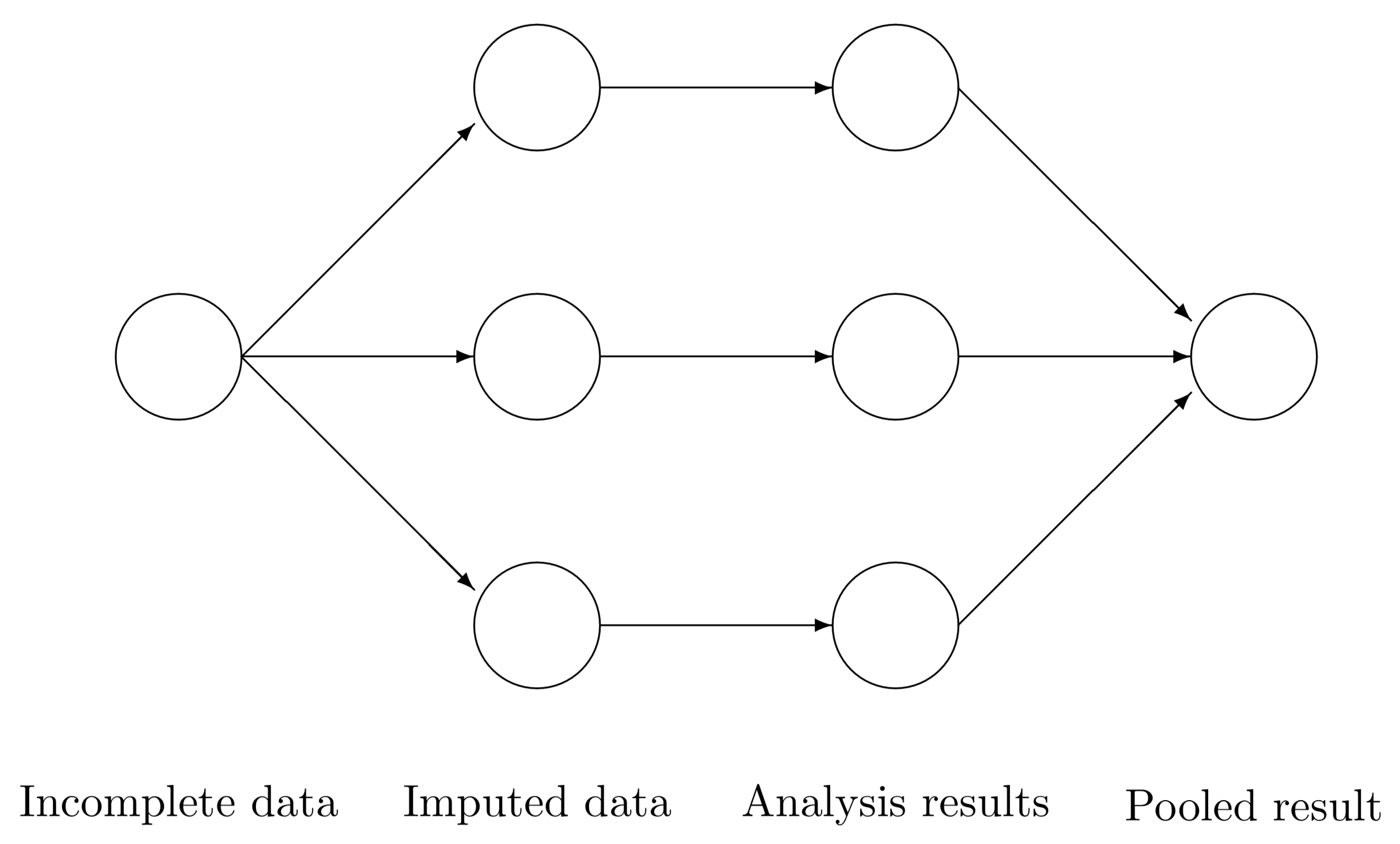
2.5. Multiple Imputation

Having explored mean and regression imputations, let us proceed to a simulation-based method called multiple imputation.

We have seen that using a single value for the imputation causes problems, such as reducing our dataset variance. Then, a handy approach is the multiple imputation method.

The idea here is, instead of imputing one value for missing data, we impute multiple values. But how can we do it?

We can do it via the mice() function, which offers this multiple imputation method. MICE stands for Multiple Imputation by Chained Equations.

Roughly speaking, for a data frame data, the four automatic steps in this R function are the following:

1. Create m copies of this dataset: data_1, data_2,…, data_m.

2. In each copy, impute the missing data with different values (the observed values will remain the same).

3. Carry out the analysis for each dataset separately. For example, fit an OLS linear regression model for each one of the datasets data_1, data_2,…,data_m when you have a continuous variable to impute.

4. Combine the separate models into one final pooled model.

We would use our pooled model, fitted with our response of interest subject to our regressor set, to answer our inferential or predictive inquiries. The below diagram provides a clearer perspective

Fig. 18 Source: van Buuren (2012).

Important

Note that the suitable regression model will be chosen accordingly depending on the nature of our variable of interest to impute. Therefore, mice() will use the following regression models:

• Binary Logistic regression for binary variables.

• Multinomial Logistic regression for categorical and nominal variables.

• Ordinal Logistic regression for categorical and ordinal variables.

We have to make sure to set up the correct variable type before imputing!

Now, how do we impute the missing data in step 2?

By default, mice() implements the predictive mean matching (PMM) found in Rubin (1987) on page 166. This is a univariate Bayesian method that does the following for each column:

1. Estimate the OLS linear regression coefficient \(\hat{\beta}_1\) and \(\hat{\sigma}\) of the column where the missing values to impute are located (as the response) versus the other column (as the regressor), using the observed complete rows only.

2. Draw \(\hat{\beta}_1^*\) and \(\hat{\sigma}^*\) using a proper posterior distribution.

3. Compute the fitted values for the column used as response in step (1), either using \(\hat{\beta}_1\) and \(\hat{\sigma}\) for those non-missing cases (i.e., \(\hat{y}_i\)) or \(\hat{\beta}_1^*\) and \(\hat{\sigma}^*\) (i.e., \(\hat{y}_i^*\)) for those missing cases.

4. For each fitted value \(\hat{y}_i^*\), we find a given number of donors (5 by default in mice()) from all the \(\hat{y}_i\)s which are the closest ones to \(\hat{y}_i^*\).

5. We randomly select one of these donors to impute the corresponding missing value.

6. The process is repeated m times.

Important

Note that this algorithm also has a multivariate version in matrix notation.

Let us implement this univariate process with sampled_flights with m = 20.

set.seed(123) # We are running a simulation, this we need to set a seed.
sampled_flights_imputed_PMM <- mice(sampled_flights, m = 20, printFlag = FALSE)
sampled_flights_imputed_PMM

Class: mids
Number of multiple imputations:  20 
Imputation methods:
dep_delay arr_delay 
    "pmm"     "pmm" 
PredictorMatrix:
          dep_delay arr_delay
dep_delay         0         1
arr_delay         1         0

We can check the imputed values for a specific column (e.g., arr_delay) in these 20 datasets as follows:

sampled_flights_imputed_PMM$imp$arr_delay

A data.frame: 407 × 20

	1	2	3	4	5	6	7	8	9	10	11	12	13	14	15	16	17	18	19	20
	<dbl>	<dbl>	<dbl>	<dbl>	<dbl>	<dbl>	<dbl>	<dbl>	<dbl>	<dbl>	<dbl>	<dbl>	<dbl>	<dbl>	<dbl>	<dbl>	<dbl>	<dbl>	<dbl>	<dbl>
1	258	92	146	218	133	82	194	179	169	138	179	243	77	113	127	104	154	99	227	108
4	127	85	100	100	97	131	131	127	97	127	85	55	92	90	85	62	90	90	97	90
5	166	185	124	111	166	308	100	90	111	222	221	163	187	158	107	195	141	100	108	107
7	113	97	195	300	270	250	162	98	127	150	238	126	100	166	129	144	116	140	273	314
8	128	103	108	158	154	153	154	105	81	80	194	102	100	100	124	324	160	84	180	181
9	162	181	101	138	117	165	117	166	160	112	115	62	187	273	170	62	107	129	161	105
17	103	128	100	125	114	160	107	127	112	213	92	62	148	215	130	80	80	80	108	100
24	107	302	82	82	153	258	112	91	132	127	131	297	181	105	125	115	123	141	110	380
28	92	81	88	317	135	158	81	243	130	158	79	152	134	100	186	218	302	82	134	172
30	127	144	228	152	107	167	195	148	218	114	190	219	160	254	258	240	130	131	102	222
⋮	⋮	⋮	⋮	⋮	⋮	⋮	⋮	⋮	⋮	⋮	⋮	⋮	⋮	⋮	⋮	⋮	⋮	⋮	⋮	⋮
975	138	114	312	148	132	137	140	160	162	112	109	209	117	285	113	119	179	92	201	292
977	100	106	274	223	119	137	104	112	114	105	130	242	98	160	119	110	152	77	143	129
979	253	176	124	161	178	317	190	158	186	178	116	116	140	131	142	140	87	308	201	115
982	158	162	127	153	143	137	215	250	81	137	244	201	160	116	91	175	201	130	183	180
985	160	315	216	161	114	132	97	90	124	136	234	189	120	92	271	139	204	150	221	98
986	62	85	97	62	97	92	62	98	97	97	90	92	98	97	98	62	92	90	90	100
991	158	104	170	108	126	109	152	118	300	149	218	69	148	149	85	153	160	139	89	250
992	100	135	128	103	98	158	122	124	111	109	124	122	120	103	128	158	158	114	128	158
993	131	201	115	114	133	100	160	137	152	112	96	257	184	167	120	131	135	323	138	130
994	174	138	158	81	124	132	110	97	131	108	110	128	166	94	98	135	157	208	103	271

Each row corresponds to a missing observation in your original dataset. The columns are the m imputed datasets that were created.

We can get each one of the m imputed datasets with complete().

# This is dataset number 3.
complete(sampled_flights_imputed_PMM, 3)

A data.frame: 1000 × 2

dep_delay	arr_delay
<dbl>	<dbl>
153	146
178	185
109	107
2	100
121	124
198	182
213	195
110	108
105	101
179	169
⋮	⋮
168	170
120	128
114	115
174	158
161	154
139	138
152	136
150	175
383	394
267	253

We can plot the imputed dataset number 3 a follows:

sampled_flights_imputed_PMM_3 <- cbind(complete(sampled_flights_imputed_PMM, 3), sampled_flights_imputed$flag)
sampled_flights_imputed_PMM_3_plot <- sampled_flights_imputed_PMM_3 %>%
  ggplot(aes(dep_delay, arr_delay)) +
  geom_point(aes(colour = flag), size = 3, alpha = .5) +
  scale_color_manual(values = c("purple", "black")) +
  theme(
    plot.title = element_text(size = 31, face = "bold"),
    axis.text = element_text(size = 21),
    axis.title = element_text(size = 27),
    legend.text = element_text(size = 21, margin = margin(r = 1, unit = "cm")),
    legend.title = element_text(size = 21, face = "bold")
  ) +
  scale_x_continuous(breaks = seq(0, 500, 100)) +
  xlab("Departure Delay (min)") +
  ylab("Arrival Delay (min)") +
  ggtitle("Complete (black) and Imputed (purple) Data")

sampled_flights_imputed_PMM_3_plot

Attention

Note this imputation method allows incomplete observations to be imputed with more realistic values, rather than just an overall mean or a fitted value coming from simple OLS regression (check purple points on top of the cloud of black points on the right-hand side). Nevertheless, it is not entirely perfect if it does not have enough complete information to impute (check purple points on the left-hand side where we do not have any complete data points in black).

Now, let us estimate an OLS linear regression for each one of the 20 imputed datasets in sampled_flights_imputed_PMM. Our response will be arr_delay subject dep_delay.

PMM_LR_models <- with(sampled_flights_imputed_PMM, lm(arr_delay ~ dep_delay))
print(PMM_LR_models)

call :
with.mids(data = sampled_flights_imputed_PMM, expr = lm(arr_delay ~ 
    dep_delay))

call1 :
mice(data = sampled_flights, m = 20, printFlag = FALSE)

nmis :
dep_delay arr_delay 
      354       407 

analyses :
[[1]]

Call:
lm(formula = arr_delay ~ dep_delay)

Coefficients:
(Intercept)    dep_delay  
    30.6428       0.8202  


[[2]]

Call:
lm(formula = arr_delay ~ dep_delay)

Coefficients:
(Intercept)    dep_delay  
    21.8563       0.8677  


[[3]]

Call:
lm(formula = arr_delay ~ dep_delay)

Coefficients:
(Intercept)    dep_delay  
    35.0526       0.8003  


[[4]]

Call:
lm(formula = arr_delay ~ dep_delay)

Coefficients:
(Intercept)    dep_delay  
     29.967        0.821  


[[5]]

Call:
lm(formula = arr_delay ~ dep_delay)

Coefficients:
(Intercept)    dep_delay  
    26.5144       0.8451  


[[6]]

Call:
lm(formula = arr_delay ~ dep_delay)

Coefficients:
(Intercept)    dep_delay  
    27.2239       0.8385  


[[7]]

Call:
lm(formula = arr_delay ~ dep_delay)

Coefficients:
(Intercept)    dep_delay  
    29.7340       0.8223  


[[8]]

Call:
lm(formula = arr_delay ~ dep_delay)

Coefficients:
(Intercept)    dep_delay  
    28.0674       0.8332  


[[9]]

Call:
lm(formula = arr_delay ~ dep_delay)

Coefficients:
(Intercept)    dep_delay  
    28.6254       0.8354  


[[10]]

Call:
lm(formula = arr_delay ~ dep_delay)

Coefficients:
(Intercept)    dep_delay  
    27.6203       0.8414  


[[11]]

Call:
lm(formula = arr_delay ~ dep_delay)

Coefficients:
(Intercept)    dep_delay  
    25.4984       0.8484  


[[12]]

Call:
lm(formula = arr_delay ~ dep_delay)

Coefficients:
(Intercept)    dep_delay  
    31.2887       0.8183  


[[13]]

Call:
lm(formula = arr_delay ~ dep_delay)

Coefficients:
(Intercept)    dep_delay  
    22.0089       0.8653  


[[14]]

Call:
lm(formula = arr_delay ~ dep_delay)

Coefficients:
(Intercept)    dep_delay  
    25.2515       0.8534  


[[15]]

Call:
lm(formula = arr_delay ~ dep_delay)

Coefficients:
(Intercept)    dep_delay  
    29.8358       0.8192  


[[16]]

Call:
lm(formula = arr_delay ~ dep_delay)

Coefficients:
(Intercept)    dep_delay  
    24.0202       0.8576  


[[17]]

Call:
lm(formula = arr_delay ~ dep_delay)

Coefficients:
(Intercept)    dep_delay  
     22.100        0.868  


[[18]]

Call:
lm(formula = arr_delay ~ dep_delay)

Coefficients:
(Intercept)    dep_delay  
    33.2085       0.8029  


[[19]]

Call:
lm(formula = arr_delay ~ dep_delay)

Coefficients:
(Intercept)    dep_delay  
    30.6784       0.8208  


[[20]]

Call:
lm(formula = arr_delay ~ dep_delay)

Coefficients:
(Intercept)    dep_delay  
    36.0514       0.7932  

We can access to each model separately as follows:

# Retrieving the third model.
PMM_LR_models$analyses[[3]]

Call:
lm(formula = arr_delay ~ dep_delay)

Coefficients:
(Intercept)    dep_delay  
    35.0526       0.8003  

Finally, let us combine the models altogether in a single pooled model.

pooled_PMM_LR_model <- pool(PMM_LR_models)
print(pooled_PMM_LR_model)

Class: mipo    m = 20 
         term  m  estimate         ubar            b            t dfcom
1 (Intercept) 20 28.262276 5.2134906153 1.668369e+01 22.731369026   998
2   dep_delay 20  0.833603 0.0001842278 5.009364e-04  0.000710211   998
        df      riv    lambda       fmi
1 28.06200 3.360105 0.7706478 0.7854151
2 30.54513 2.855070 0.7406014 0.7560670

The estimate column is just the averages of all m models. Full details about the computation on these columns are provided by Rubin (1987) on pages 76 and 77. The columns are explained as follows:

• estimate: the average of the regression coefficients across m models.

• ubar: the average variance (i.e., average SE^2) across m models.

• b: the sample variance of the m regression coefficients.

• t: a final estimate of the SE^2 of each regression coefficient.

  • = ubar + (1 + 1/m) * b

• dfcom: the degrees of freedom associated with the final regression coefficient estimates.

  • An alpha-level confidence interval: estimate +/- qt(alpha/2, df) * sqrt(t).

• riv: the relative increase in variance due to randomness.

  • = t/ubar - 1

• lambda: the proportion of total variance due to missingness.

• fmi: the fraction of missing information.

Where are the usual outputs (std.error, p.value,…)?

We can call summary() on the pooled model to obtain them. The usual coefficient interpretations and inferential rules also apply in this pooled OLS model.

summary(pooled_PMM_LR_model)

A mipo.summary: 2 × 6

term	estimate	std.error	statistic	df	p.value
<fct>	<dbl>	<dbl>	<dbl>	<dbl>	<dbl>
(Intercept)	28.262276	4.76774255	5.927811	28.06200	2.203849e-06
dep_delay	0.833603	0.02664978	31.279914	30.54513	9.205948e-25

3. Wrapping Up

• Data imputation involves some wrangling effort and proper missingness visualizations.

• We have to be careful when defining our class of data missingness since this will determine the type of data imputation we need to make (or maybe data deletion!).

• In general, multiple imputation will work OK for MAR and MNAR data.

• We only saw continuous imputation in this example. Nonetheless, the mice() approach can be extended to other data types such as binary or categorical. In those cases, we have to switch to generalized linear models (GLMs), even with a Bayesian approach.